Download the notebook here! Interactive online version:

Portfolio optimization

In the Measure Impact stage we produced causal estimates. In the Evaluate Evidence stage we assessed how much to trust them. This lecture addresses the final question: given confidence-weighted return estimates for a set of initiatives, which ones should we fund?

The answer requires decision theory. An organization faces a binary selection problem — fund or skip each initiative — subject to a budget constraint, with returns that depend on an unknown state of nature. The confidence scores from the EVALUATE stage enter directly. Lower confidence penalizes an initiative’s projected returns, pulling them toward the worst case. This creates a built-in incentive for better measurement. Investing in evidence quality raises an initiative’s effective returns and improves its chances of selection.

Part I develops the mathematical framework following Eisenhauer (2025). Part II applies it end-to-end using the impact-engine-allocate package on mock portfolio data matching the paper’s simulation example.

---

Part I: theory

1. The decision problem

An organization has \(N\) investment initiatives indexed by the set \(I = \{1, \ldots, N\}\). Each initiative \(i\) has a known cost \(b_i\) and an uncertain return that depends on which scenario materializes. The total budget is \(B\).

The decision is binary: for each initiative \(i\), the decision variable \(x_i \in \{0, 1\}\) indicates whether to fund it. The portfolio vector \(\mathbf{x} = (x_1, \ldots, x_N)\) collects all selection decisions. The constraints are:

\[x_i \in \{0, 1\} \quad \forall i \in I \tag{2}\]

\[\sum_{i=1}^{N} b_i x_i \leq B \tag{5}\]

Equation (2) makes the problem a binary integer program — each initiative is either fully funded or not. Equation (5) ensures total spending does not exceed the budget. The objective function depends on the decision rule, which we develop in §4 and §5.

2. Scenario-dependent returns

Returns are uncertain because they depend on which state of nature materializes. The set of scenarios \(S = \{s_1, \ldots, s_M\}\) represents the possible states. In the standard configuration, \(S = \{s_{\text{best}}, s_{\text{med}}, s_{\text{worst}}\}\) — three scenarios spanning the range of plausible outcomes.

For each initiative \(i\) and scenario \(s_j\), the baseline return \(R_{ij}\) captures the net return (revenue minus cost) if \(i\) is funded and scenario \(s_j\) materializes. The worst-case return across all scenarios defines a floor:

\[R_i^{\min} = \min_{s_j \in S} R_{ij}\]

These baseline returns come from the MEASURE stage — they are the causal effect estimates produced by the Impact Engine. The key question is how much to trust them, which is where the EVALUATE stage enters.

3. The confidence penalty

The confidence score \(c_i \in [0, 1]\) from the EVALUATE stage quantifies how much to trust initiative \(i\)’s return estimates. A low confidence score means the evidence is weak — the true returns could be far from the estimates. The framework translates this epistemic uncertainty into a penalty on projected returns.

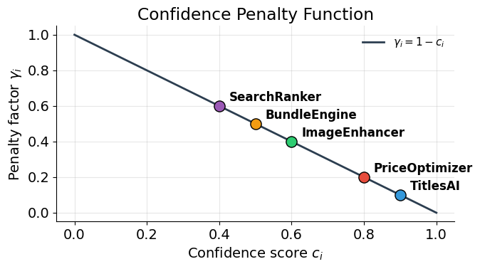
The penalty factor \(\gamma_i\) decreases monotonically with confidence:

\[\gamma_i = f(c_i) = 1 - c_i\]

Each scenario return blends toward the worst case, weighted by the penalty. The resulting effective return \(\tilde{R}_{ij}\) reflects both the projected outcome and the quality of evidence behind it:

\[\tilde{R}_{ij} = (1 - \gamma_i) R_{ij} + \gamma_i R_i^{\min} \quad \forall s_j \in S\]

When confidence is perfect (\(c_i = 1\), \(\gamma_i = 0\)), the effective return equals the baseline: \(\tilde{R}_{ij} = R_{ij}\). When confidence is zero (\(c_i = 0\), \(\gamma_i = 1\)), all scenarios collapse to the worst case: \(\tilde{R}_{ij} = R_i^{\min}\). This creates a direct incentive for better measurement — improving evidence quality raises an initiative’s effective returns.

A minimum confidence threshold \(c_{\min}\) excludes initiatives with insufficient evidence:

\[c_i \geq c_{\min} \cdot x_i \quad \forall i \in I \tag{3}\]

Any initiative with \(c_i < c_{\min}\) is ineligible for selection regardless of its projected returns.

4. Minimax regret optimization

The minimax regret rule selects the portfolio that minimizes the worst-case disappointment across all scenarios. Defining regret requires an optimal benchmark — the best achievable effective return under each scenario:

\[V_j^* = \max_{\mathbf{x}} \sum_{i=1}^{N} \tilde{R}_{ij} x_i \quad \text{s.t. budget and binary constraints}\]

The regret of portfolio \(\mathbf{x}\) under scenario \(s_j\) measures the gap between what was achievable and what the portfolio delivers:

\[\text{Regret}_j(\mathbf{x}) = V_j^* - \sum_{i=1}^{N} \tilde{R}_{ij} x_i\]

The minimax regret formulation introduces an auxiliary variable \(\theta\) that bounds the maximum regret:

\[\min_{\mathbf{x}, \theta} \quad \theta \tag{1}\]

\[\theta \geq V_j^* - \sum_{i=1}^{N} \tilde{R}_{ij} x_i \quad \forall s_j \in S \tag{4}\]

subject to the binary constraint (2), the confidence threshold (3), and the budget constraint (5). An optional downside safeguard guarantees a minimum portfolio return under the worst case:

\[\sum_{i=1}^{N} R_i^{\min} x_i \geq R_{\min}^{\text{portfolio}} \tag{6}\]

The minimax regret rule is conservative — it protects against the scenario where the chosen portfolio performs worst relative to what was possible. The optimal \(\theta^*\) tells the decision-maker the maximum regret they face.

5. Bayesian decision rule

An alternative to minimax regret is the Bayesian decision rule, which assigns probability weights \(w_j\) to each scenario and maximizes the weighted expected return:

\[\max_{\mathbf{x}} \sum_{j=1}^{M} w_j \sum_{i=1}^{N} \tilde{R}_{ij} x_i\]

subject to the same constraints (2), (3), (5), and (6). The weights satisfy \(w_j \geq 0\) and \(\sum_j w_j = 1\).

Different weight profiles express different beliefs about which scenario is most likely:

Profile	\(w_{\text{best}}\)	\(w_{\text{med}}\)	\(w_{\text{worst}}\)	Interpretation
Optimistic	0.50	0.30	0.20	Upside scenarios dominate
Balanced	0.33	0.34	0.33	Equal uncertainty across scenarios
Pessimistic	0.20	0.30	0.50	Worst case most likely

The Bayesian rule is less conservative than minimax regret — it allows the decision-maker to express beliefs about scenario likelihoods rather than optimizing for the worst case. Comparing the two rules on the same portfolio reveals how much the portfolio choice depends on the decision-maker’s attitude toward uncertainty.

---

Part II: application

# Standard Library
import copy
import inspect

# Third-party
import pandas as pd
import yaml
from impact_engine_allocate import BayesianAllocation, MinimaxRegretAllocation
from impact_engine_allocate.allocation import (
    calculate_effective_returns,
    calculate_gamma,
    preprocess,
)
from IPython.display import Code

# Local
from support import (
    create_mock_portfolio,
    display_solver_result,
    plot_confidence_penalty,
    plot_effective_return_interpolation,
    plot_effective_returns_heatmap,
    plot_penalty_curve,
    plot_portfolio_comparison,
    plot_scenario_returns_with_regret,
    plot_selection_matrix,
    plot_sensitivity_analysis,
)

1. Initiative data

We construct a mock portfolio of five initiatives matching the simulation example in Eisenhauer (2025), Table 1. Each initiative has a cost, three scenario returns (best, median, worst), and a confidence score from the EVALUATE stage. Using the paper’s exact values lets us verify Part II results against the published tables.

Code(inspect.getsource(create_mock_portfolio), language="python")

def create_mock_portfolio():
    """
    Create a portfolio of five initiatives matching the paper's Table 1.

    Returns a list of initiative dicts with the keys expected by
    ``impact_engine_allocate``: ``id``, ``cost``, ``R_best``, ``R_med``,
    ``R_worst``, and ``confidence``.

    Returns
    -------
    list[dict]
        Five initiatives with costs, scenario returns, and confidence
        scores from Eisenhauer (2025), Table 1.
    """
    return [
        {"id": "TitlesAI", "cost": 4, "R_best": 15, "R_med": 10, "R_worst": 2, "confidence": 0.90},
        {"id": "ImageEnhancer", "cost": 2, "R_best": 12, "R_med": 8, "R_worst": 1, "confidence": 0.60},
        {"id": "PriceOptimizer", "cost": 2, "R_best": 9, "R_med": 6, "R_worst": 2, "confidence": 0.80},
        {"id": "SearchRanker", "cost": 2, "R_best": 7, "R_med": 5, "R_worst": 3, "confidence": 0.40},
        {"id": "BundleEngine", "cost": 4, "R_best": 18, "R_med": 9, "R_worst": 0, "confidence": 0.50},
    ]

initiatives = create_mock_portfolio()

df = pd.DataFrame(initiatives)
df["gamma"] = df["confidence"].apply(calculate_gamma)
df

	id	cost	R_best	R_med	R_worst	confidence	gamma
0	TitlesAI	4	15	10	2	0.9	0.1
1	ImageEnhancer	2	12	8	1	0.6	0.4
2	PriceOptimizer	2	9	6	2	0.8	0.2
3	SearchRanker	2	7	5	3	0.4	0.6
4	BundleEngine	4	18	9	0	0.5	0.5

TitlesAI has the highest confidence (\(c = 0.90\), \(\gamma = 0.10\)) — its evidence is strong, so the penalty is minimal. SearchRanker has the lowest confidence (\(c = 0.40\), \(\gamma = 0.60\)) and will be excluded by the confidence threshold. BundleEngine has large upside (\(R_{\text{best}} = 18\)) but zero downside (\(R_{\text{worst}} = 0\)) and medium confidence (\(c = 0.50\)).

2. Configuration

The allocation parameters are stored in "config_allocation.yaml". The configuration specifies three constraints: the total budget, the minimum confidence threshold for eligibility, and the minimum worst-case portfolio return (the downside safeguard from Part I, equation 6).

! cat config_allocation.yaml

total_budget: 10
min_confidence_threshold: 0.50
min_portfolio_worst_return: 3

with open("config_allocation.yaml") as f:
    config = yaml.safe_load(f)

3. The confidence penalty

The function calculate_effective_returns() computes \(\gamma_i\) and the effective returns \(\tilde{R}_{ij}\) for each initiative.

initiatives_with_returns = calculate_effective_returns(initiatives)

rows = []
for init in initiatives_with_returns:
    eff = init["effective_returns"]
    rows.append(
        {
            "id": init["id"],
            "gamma": init["gamma"],
            "R_best_eff": eff["best"],
            "R_med_eff": eff["med"],
            "R_worst_eff": eff["worst"],
        }
    )
pd.DataFrame(rows).set_index("id")

	gamma	R_best_eff	R_med_eff	R_worst_eff
id
TitlesAI	0.1	13.7	9.2	2.0
ImageEnhancer	0.4	7.6	5.2	1.0
PriceOptimizer	0.2	7.6	5.2	2.0
SearchRanker	0.6	4.6	3.8	3.0
BundleEngine	0.5	9.0	4.5	0.0

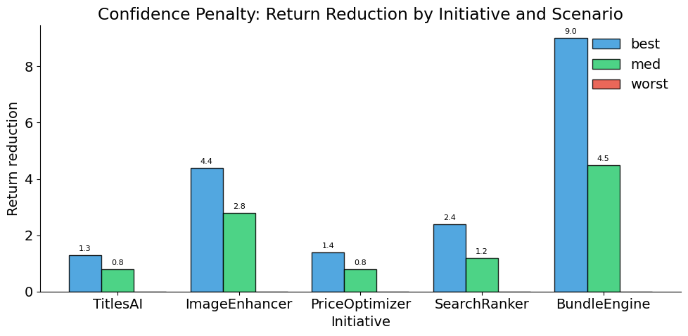
plot_confidence_penalty(initiatives_with_returns)

plot_penalty_curve(initiatives)

The plot below shows how BundleEngine’s effective returns vary as confidence moves from 0 to 1. Each line represents one scenario. The vertical dashed line marks BundleEngine’s actual confidence score, and the dots show its current effective returns.

plot_effective_return_interpolation(initiatives[4])

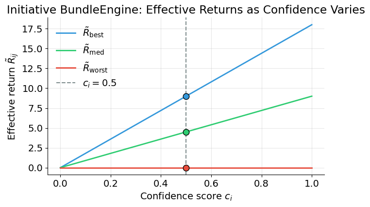
The penalty hits BundleEngine hardest (\(\gamma = 0.50\)): its best-case effective return drops from 18 to 9.0 because half the return is pulled toward the worst case of 0. TitlesAI’s returns barely change (\(\gamma = 0.10\)) — strong evidence preserves projected returns.

4. Preprocessing

The preprocess() function filters initiatives below the confidence threshold and computes effective returns for the remaining ones.

processed = preprocess(initiatives, min_confidence_threshold=config["min_confidence_threshold"])

print(f"Initiatives before preprocessing: {len(initiatives)}")
print(f"Initiatives after preprocessing:  {len(processed)}")
print(f"Excluded: {[init['id'] for init in initiatives if init['id'] not in [p['id'] for p in processed]]}")

Initiatives before preprocessing: 5
Initiatives after preprocessing:  4
Excluded: ['SearchRanker']

plot_effective_returns_heatmap(processed)

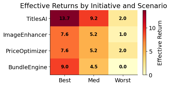
SearchRanker (\(c = 0.40\)) falls below the \(c_{\min} = 0.50\) threshold and is excluded. Four initiatives remain eligible: TitlesAI, ImageEnhancer, PriceOptimizer, and BundleEngine.

5. From theory to code

The "config_allocation.yaml" fields map directly to the theoretical constructs from Part I. The table below connects each configuration parameter to its role in the optimization formulation.

Config Field	Part I Concept
total_budget	Total available resources \(B\) (equation 5)
min_confidence_threshold	Minimum confidence threshold \(c_{\min}\) (equation 3)
min_portfolio_worst_return	Downside safeguard \(R_{\min}^{\text{portfolio}}\) (equation 6)

The initiative data fields map to the mathematical objects:

Initiative Field	Part I Concept
id	Initiative index \(i \in I\)
cost	Cost \(b_i\)
R_best, R_med, R_worst	Baseline returns \(R_{ij}\) under each scenario \(s_j \in S\)
confidence	Confidence score \(c_i\) from the EVALUATE stage
gamma	Penalty factor \(\gamma_i = 1 - c_i\)
effective_returns	Confidence-adjusted returns \(\tilde{R}_{ij}\)

6. Minimax regret

MinimaxRegretAllocation solves the binary integer program from Part I, §4. It takes the preprocessed initiatives and returns the portfolio that minimizes worst-case regret across all scenarios.

minimax_solver = MinimaxRegretAllocation()
minimax_result = minimax_solver(
    processed,
    total_budget=config["total_budget"],
    min_portfolio_worst_return=config["min_portfolio_worst_return"],
)

display_solver_result(minimax_result, "Minimax regret")

Minimax regret
==================================================
  Status:     Optimal
  Selected:   ['TitlesAI', 'PriceOptimizer', 'BundleEngine']
  Total cost: 10.0
  Objective:  1.00

  Portfolio returns by scenario:
     best: 30.3
      med: 18.9
    worst: 4.0

The solver selects TitlesAI, PriceOptimizer, and BundleEngine at a total cost of 10 (exactly exhausting the budget). The maximum regret \(\theta^* = 1.0\) means that in no scenario does this portfolio fall more than 1.0 below what was achievable. ImageEnhancer is excluded despite being eligible — its inclusion would exceed the budget.

plot_scenario_returns_with_regret(minimax_result, "Minimax Regret: Regret Gaps by Scenario")

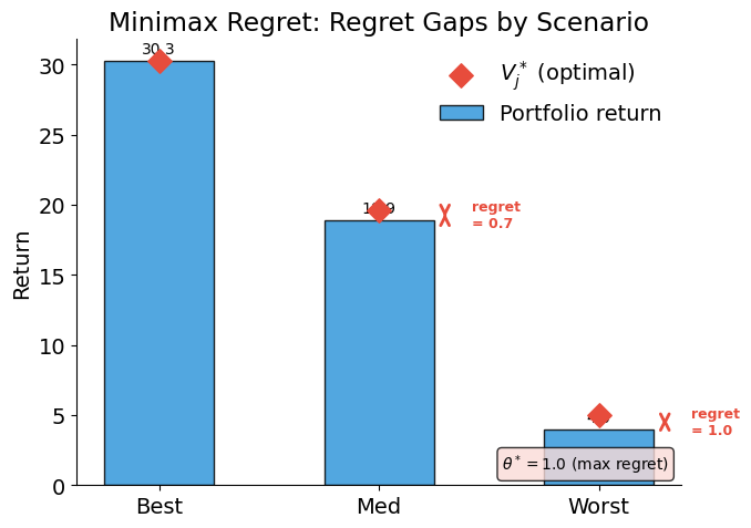
The diamond markers show the optimal benchmark \(V_j^*\) for each scenario — the best return achievable under budget constraints if we could pick the portfolio knowing which scenario would materialize. The gap between the bar and the diamond is the regret. Minimax regret minimizes the largest such gap across all scenarios.

7. Bayesian allocation

The Bayesian decision rule from Part I, §5 maximizes weighted expected return. We solve with three weight profiles expressing different beliefs about scenario likelihoods.

weight_profiles = {
    "Optimistic": {"best": 0.50, "med": 0.30, "worst": 0.20},
    "Balanced": {"best": 0.33, "med": 0.34, "worst": 0.33},
    "Pessimistic": {"best": 0.20, "med": 0.30, "worst": 0.50},
}

bayesian_results = {}
for name, weights in weight_profiles.items():
    solver = BayesianAllocation(weights)
    result = solver(
        processed,
        total_budget=config["total_budget"],
        min_portfolio_worst_return=config["min_portfolio_worst_return"],
    )
    bayesian_results[name] = result
    display_solver_result(result, f"Bayesian ({name.lower()})")
    print()

Bayesian (optimistic)
==================================================
  Status:     Optimal
  Selected:   ['TitlesAI', 'PriceOptimizer', 'BundleEngine']
  Total cost: 10.0
  Objective:  21.62

  Portfolio returns by scenario:
     best: 30.3
      med: 18.9
    worst: 4.0

Bayesian (balanced)
==================================================
  Status:     Optimal
  Selected:   ['TitlesAI', 'ImageEnhancer', 'PriceOptimizer']
  Total cost: 8.0
  Objective:  17.85

  Portfolio returns by scenario:
     best: 28.9
      med: 19.6
    worst: 5.0

Bayesian (pessimistic)
==================================================
  Status:     Optimal
  Selected:   ['TitlesAI', 'ImageEnhancer', 'PriceOptimizer']
  Total cost: 8.0
  Objective:  14.16

  Portfolio returns by scenario:
     best: 28.9
      med: 19.6
    worst: 5.0

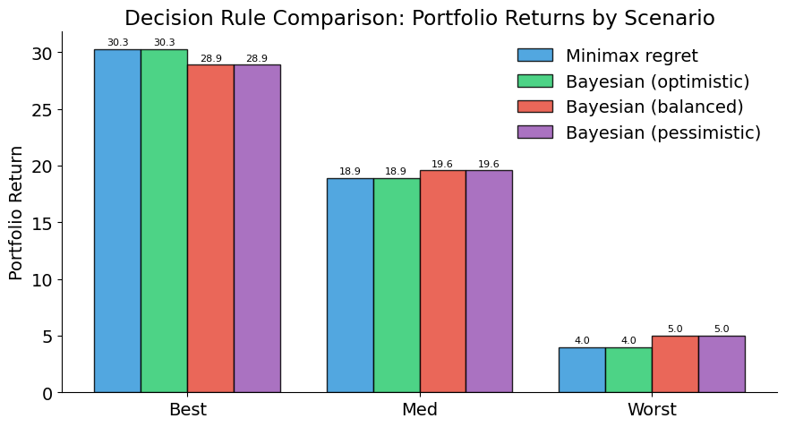
8. Comparing decision rules

The comparison reveals how portfolio choice depends on the decision-maker’s attitude toward uncertainty.

all_results = [("Minimax regret", minimax_result)]
for name, result in bayesian_results.items():
    all_results.append((f"Bayesian ({name.lower()})", result))

plot_portfolio_comparison(all_results)

print("Selected initiatives by decision rule")
print("=" * 50)
for name, result in all_results:
    selected = result["selected_initiatives"]
    cost = result["total_cost"]
    print(f"  {name + ':':30s} {selected}  (cost={cost:.0f})")

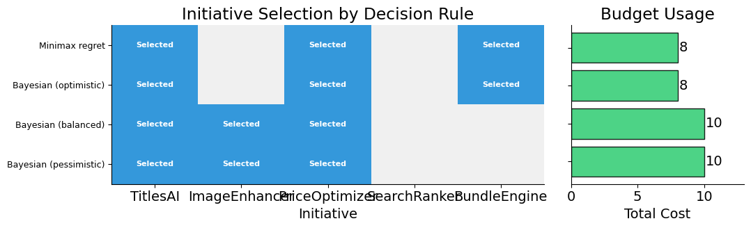
Selected initiatives by decision rule
==================================================
  Minimax regret:                ['TitlesAI', 'PriceOptimizer', 'BundleEngine']  (cost=10)
  Bayesian (optimistic):         ['TitlesAI', 'PriceOptimizer', 'BundleEngine']  (cost=10)
  Bayesian (balanced):           ['TitlesAI', 'ImageEnhancer', 'PriceOptimizer']  (cost=8)
  Bayesian (pessimistic):        ['TitlesAI', 'ImageEnhancer', 'PriceOptimizer']  (cost=8)

plot_selection_matrix(all_results, [init["id"] for init in initiatives])

9. How confidence shapes allocation

The confidence penalty creates a direct link between evidence quality and resource allocation. We vary BundleEngine’s confidence downward from 0.90 to 0.10 and observe how the minimax regret solution changes. BundleEngine is currently selected with confidence 0.50 — what happens as evidence quality deteriorates further?

confidence_values = [0.90, 0.80, 0.70, 0.60, 0.50, 0.45, 0.40, 0.30, 0.20, 0.10]

print("Effect of BundleEngine's confidence on minimax regret solution")
print("=" * 75)
print(f"  {'c':>5s}  {'gamma':>5s}  {'Selected':>45s}  {'theta*':>7s}  {'Worst return':>13s}")
print("-" * 75)

for c_val in confidence_values:
    modified = copy.deepcopy(initiatives)
    for init in modified:
        if init["id"] == "BundleEngine":
            init["confidence"] = c_val

    modified_processed = preprocess(modified, min_confidence_threshold=config["min_confidence_threshold"])
    result = minimax_solver(
        modified_processed,
        total_budget=config["total_budget"],
        min_portfolio_worst_return=config["min_portfolio_worst_return"],
    )

    selected = ", ".join(result["selected_initiatives"])
    theta = result["objective_value"]
    worst = result["total_actual_returns"].get("worst", 0.0)
    gamma_val = calculate_gamma(c_val)
    theta_str = f"{theta:.2f}" if theta is not None else "N/A"
    print(f"  {c_val:5.2f}  {gamma_val:5.2f}  {selected:>45s}  {theta_str:>7s}  {worst:13.1f}")

Effect of BundleEngine's confidence on minimax regret solution
===========================================================================
      c  gamma                                       Selected   theta*   Worst return
---------------------------------------------------------------------------
   0.90   0.10         TitlesAI, PriceOptimizer, BundleEngine     1.00            4.0
   0.80   0.20         TitlesAI, PriceOptimizer, BundleEngine     1.00            4.0
   0.70   0.30         TitlesAI, PriceOptimizer, BundleEngine     1.00            4.0
   0.60   0.40         TitlesAI, PriceOptimizer, BundleEngine     1.00            4.0
   0.50   0.50         TitlesAI, PriceOptimizer, BundleEngine     1.00            4.0
   0.45   0.55        TitlesAI, ImageEnhancer, PriceOptimizer     0.00            5.0
   0.40   0.60        TitlesAI, ImageEnhancer, PriceOptimizer     0.00            5.0
   0.30   0.70        TitlesAI, ImageEnhancer, PriceOptimizer     0.00            5.0
   0.20   0.80        TitlesAI, ImageEnhancer, PriceOptimizer     0.00            5.0
   0.10   0.90        TitlesAI, ImageEnhancer, PriceOptimizer     0.00            5.0

sensitivity_data = []

for c_val in confidence_values:
    modified = copy.deepcopy(initiatives)
    for init in modified:
        if init["id"] == "BundleEngine":
            init["confidence"] = c_val

    modified_processed = preprocess(modified, min_confidence_threshold=config["min_confidence_threshold"])
    result = minimax_solver(
        modified_processed,
        total_budget=config["total_budget"],
        min_portfolio_worst_return=config["min_portfolio_worst_return"],
    )

    sensitivity_data.append(
        {
            "c_e": c_val,
            "gamma": calculate_gamma(c_val),
            "theta": result["objective_value"],
            "worst_return": result["total_actual_returns"].get("worst", 0.0),
            "selected": result["selected_initiatives"],
        }
    )

plot_sensitivity_analysis(sensitivity_data, initiative_label="BundleEngine")

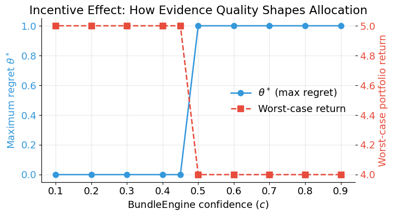
As confidence in BundleEngine’s evidence deteriorates, its effective returns drop. Once confidence falls below the \(c_{\min} = 0.50\) threshold, BundleEngine becomes ineligible and the solver selects a different portfolio. Better measurement does not just improve estimates — it determines which initiatives get funded.

Additional resources

• Eisenhauer, P. (2025). Science-backed decisions for high-stakes investments under uncertainty. Working paper.

• eisenhauer.io (2026). impact-engine-allocate documentation. Usage, configuration, and system design.