Download the notebook here! Interactive online version:

Potential Outcomes Model

Reference: Causal Inference: The Mixtape, Chapter 4: Potential Outcomes Causal Model (pp. 119-174)

This lecture introduces the potential outcome framework for causal inference. We apply these concepts using the Online Retail Simulator to answer: What would be the effect on sales if we improved product content quality?

---

Part I: Theory

This section covers the theoretical foundations of the potential outcome framework as presented in Cunningham’s Causal Inference: The Mixtape, Chapter 4.

1. The potential outcome framework

The potential outcome framework, also known as the Rubin Causal Model (RCM), provides a precise mathematical language for defining causal effects. The framework was developed by Donald Rubin in the 1970s, building on earlier work by Jerzy Neyman.

Core definitions

For each unit \(i\) in a population, we define:

• \(D_i \in \{0, 1\}\): Treatment indicator (1 if unit receives treatment, 0 otherwise)

• \(Y_i^1\): Potential outcome under treatment — the outcome unit \(i\) would have if treated

• \(Y_i^0\): Potential outcome under control — the outcome unit \(i\) would have if not treated

The key insight is that both potential outcomes exist conceptually for every unit, but we can only observe one of them.

The switching equation

The observed outcome follows the switching equation:

\[Y_i = D_i \cdot Y_i^1 + (1 - D_i) \cdot Y_i^0\]

This equation formalizes which potential outcome we observe:

• If \(D_i = 1\) (treated): we observe \(Y_i = Y_i^1\)

• If \(D_i = 0\) (control): we observe \(Y_i = Y_i^0\)

Individual treatment effects

The individual treatment effect (ITE) for unit \(i\) is defined as:

\[\delta_i = Y_i^1 - Y_i^0\]

This measures how much unit \(i\)’s outcome would change due to treatment.

2. SUTVA: stable unit treatment value assumption

The switching equation assumes that unit \(i\)’s observed outcome depends only on its own treatment, and that treatment means the same thing for every unit. This is the stable unit treatment value assumption (SUTVA), which has two components:

1. No interference

One unit’s treatment assignment does not affect another unit’s potential outcomes:

\[Y_i^d = Y_i^d(D_1, D_2, \ldots, D_n) \text{ depends only on } D_i\]

Violations:

• Vaccine trials: Your vaccination protects others (herd immunity)

• Classroom interventions: Tutoring one student may help their study partners

• Market interventions: Promoting one product may cannibalize another

2. No hidden variations in treatment

Treatment is well-defined — there is only one version of “treatment” and one version of “control”:

\[Y_i^1 \text{ is the same regardless of how treatment is administered}\]

Violations:

• Drug dosage varies across treated patients

• Job training programs have different instructors

• “Content optimization” could mean different things for different products

3. The fundamental problem of causal inference

Holland (1986) articulated what he called the fundamental problem of causal inference: we cannot observe both potential outcomes for the same unit at the same time.

Consider this example:

Unit	Treatment	Observed	\(Y^1\)	\(Y^0\)
A	Treated	$500	$500	?
B	Control	$300	?	$300
C	Treated	$450	$450	?
D	Control	$280	?	$280

The question marks represent counterfactuals — outcomes that would have occurred under the alternative treatment assignment. These are fundamentally unobservable.

This is not a data limitation that can be solved with more observations or better measurement. It is a logical impossibility: the same unit cannot simultaneously exist in both treatment states.

It follows that the individual treatment effect \(\delta_i\) can never be computed for any unit. This is why causal inference focuses on population-level parameters instead.

4. Population-level parameters

Since individual effects are unobservable, we focus on population averages:

Parameter	Definition	Interpretation
ATE	\(E[Y^1 - Y^0]\)	Average effect across all units
ATT	\(E[Y^1 - Y^0 \mid D=1]\)	Average effect among units that were treated
ATC	\(E[Y^1 - Y^0 \mid D=0]\)	Average effect among units that were not treated

When do these differ?

If treatment effects are homogeneous (same for everyone), then \(\text{ATE} = \text{ATT} = \text{ATC}\).

If treatment effects are heterogeneous and correlated with treatment selection, these parameters will differ. For example, if high-ability workers are more likely to get job training and benefit more from it, then \(\text{ATT} > \text{ATE}\).

5. The naive estimator and selection bias

The most intuitive approach to estimating causal effects is the naive estimator (also called the simple difference in means):

\[\hat{\delta}_{\text{naive}} = E[Y \mid D=1] - E[Y \mid D=0]\]

This compares average outcomes between treated and control groups. When does this equal the ATE?

Decomposing the naive estimator

Adding and subtracting \(E[Y^0 \mid D=1]\) and the ATE splits the naive estimator into the ATE and two sources of bias:

\[\hat{\delta}_{\text{naive}} = \underbrace{E[Y^1 - Y^0]}_{\text{ATE}} + \underbrace{E[Y^0 \mid D=1] - E[Y^0 \mid D=0]}_{\text{Baseline Bias}} + \underbrace{E[\delta \mid D=1] - E[\delta]}_{\text{Differential Treatment Effect Bias}}\]

• Baseline bias (selection bias): treated units would have had different outcomes than control units even without treatment

• Differential treatment effect bias: treated units benefit more or less from treatment than the average unit, so \(\text{ATT} \neq \text{ATE}\)

The naive estimator equals the ATE only when both terms are zero.

The special case of homogeneous effects

When the treatment effect is the same for every unit, \(\text{ATT} = \text{ATE}\) and the second term vanishes:

\[E[Y \mid D=1] - E[Y \mid D=0] = \text{ATE} + \underbrace{E[Y^0 \mid D=1] - E[Y^0 \mid D=0]}_{\text{Selection Bias}}\]

This is the version most often quoted, but it hides the second source of bias whenever effects are heterogeneous.

6. Randomization: the gold standard

Randomized controlled trials (RCTs) solve the selection bias problem by ensuring treatment is assigned independently of potential outcomes.

Independence assumption

Under randomization:

\[(Y^1, Y^0) \perp\!\!\!\perp D\]

This means potential outcomes are statistically independent of treatment assignment.

Why randomization works

Under independence:

\[E[Y^0 \mid D=1] = E[Y^0 \mid D=0] = E[Y^0]\]

\[E[Y^1 \mid D=1] = E[Y^1 \mid D=0] = E[Y^1]\]

Therefore:

\[E[Y \mid D=1] - E[Y \mid D=0] = E[Y^1] - E[Y^0] = \text{ATE}\]

Both bias terms vanish: baseline bias because \(E[Y^0 \mid D=1] = E[Y^0 \mid D=0]\), and differential treatment effect bias because \(E[\delta \mid D=1] = E[\delta]\). The naive estimator becomes unbiased under randomization.

---

Part II: Application

In Part I we defined the potential outcome framework: individual treatment effects \(\delta_i = Y_i^1 - Y_i^0\), population parameters (ATE, ATT, ATC), and the decomposition showing how selection bias corrupts the naive estimator. We also saw that randomization eliminates selection bias by making treatment independent of potential outcomes.

In this application, the simulator gives us an omniscient view — we observe both potential outcomes for every product. This lets us compute true treatment effects, verify the bias decomposition numerically, and demonstrate that randomization recovers the truth.

# Standard library
import inspect

# Third-party packages
import numpy as np
import pandas as pd
from IPython.display import Code
from online_retail_simulator import simulate, load_job_results
from online_retail_simulator.enrich import enrich
from online_retail_simulator.enrich.enrichment_library import quantity_boost

# Local imports
from support import (
    create_confounded_treatment,
    difference_in_means,
    generate_quality_score,
    plot_balance_check,
    plot_individual_effects_distribution,
    plot_randomization_comparison,
    plot_sample_size_convergence,
    print_bias_decomposition,
    print_ite_summary,
    print_naive_estimator,
    random_assignment,
)

# One random number generator drives every random step in this notebook
rng = np.random.default_rng(42)

1. Business context

What would be the effect on sales if we improved product content quality?

An e-commerce company is considering investing in content optimization (better descriptions, images, etc.) for its product catalog. Before rolling this out to all products, they want to understand the causal effect of content optimization on revenue.

The challenge is a selection paradox: the company targets the weakest products for optimization — a sensible business decision — but this strategic selection makes the treated group look worse than the control group even before any treatment, confounding the naive comparison.

In our simulation:

Variable	Notation	Description
Treatment	\(D=1\)	Product receives content optimization
Control	\(D=0\)	Product keeps original content
Outcome	\(Y\)	Product revenue

2. Data and assignment mechanism

We simulate 5,000 products with a single day of sales data. The simulation produces baseline metrics, from which we derive a quality score and assign treatment. The company selects the lowest-quality 30% of products for content optimization — a realistic business decision to invest where the need is greatest. This strategic selection creates confounding: treated products already had lower baseline revenue before any optimization.

!cat "config_simulation.yaml"

STORAGE:
  PATH: output

RULE:
  PRODUCTS:
    FUNCTION: simulate_products_rule_based
    PARAMS:
      num_products: 5000
      seed: 42

  METRICS:
    FUNCTION: simulate_metrics_rule_based
    PARAMS:
      date_start: "2024-11-15"
      date_end: "2024-11-15"
      sale_prob: 0.7
      seed: 42

PRODUCT_DETAILS:
  FUNCTION: simulate_product_details_mock

# Run simulation and load baseline metrics
job_info = simulate("config_simulation.yaml")
metrics = load_job_results(job_info)["metrics"]

print(f"Metrics records: {len(metrics)}")
print(f"Unique products: {metrics['product_identifier'].nunique()}")

Metrics records: 5000
Unique products: 5000

Code(inspect.getsource(create_confounded_treatment), language="python")

def create_confounded_treatment(metrics_df, treatment_fraction=0.3, true_effect=0.5, seed=42):
    """
    Create confounded treatment assignment from raw simulator metrics.

    Aggregates revenue per product, generates a quality score, then assigns
    treatment deterministically to the lowest-quality products (struggling
    products get optimized). This creates negative selection bias: treated
    products have lower baseline revenue.

    Parameters
    ----------
    metrics_df : pandas.DataFrame
        Metrics DataFrame with ``product_identifier`` and ``revenue`` columns.
    treatment_fraction : float, optional
        Fraction of products to treat (selected from the bottom by quality).
    true_effect : float, optional
        True causal effect of treatment (proportional increase in revenue).
    seed : int or numpy.random.Generator, optional
        Random seed or generator for reproducibility.

    Returns
    -------
    pandas.DataFrame
        DataFrame with columns ``product_identifier``, ``quality_score``,
        ``D``, ``Y0``, ``Y1``, ``Y_observed``.
    """
    product_revenue = metrics_df.groupby("product_identifier")["revenue"].sum().reset_index()
    product_revenue.columns = ["product_identifier", "baseline_revenue"]

    product_revenue["quality_score"] = generate_quality_score(product_revenue["baseline_revenue"], seed=seed)

    # Treat bottom fraction by quality (struggling products get optimized)
    n_treat = int(len(product_revenue) * treatment_fraction)
    treated_ids = set(product_revenue.nsmallest(n_treat, "quality_score")["product_identifier"])
    product_revenue["D"] = product_revenue["product_identifier"].isin(treated_ids).astype(int)

    # Potential outcomes
    product_revenue["Y0"] = product_revenue["baseline_revenue"]
    product_revenue["Y1"] = product_revenue["baseline_revenue"] * (1 + true_effect)
    product_revenue["Y_observed"] = np.where(product_revenue["D"] == 1, product_revenue["Y1"], product_revenue["Y0"])

    return product_revenue[["product_identifier", "quality_score", "D", "Y0", "Y1", "Y_observed"]]

# Apply the confounded treatment assignment
TRUE_EFFECT = 0.5  # 50% revenue boost from content optimization

confounded_products = create_confounded_treatment(
    metrics,
    treatment_fraction=0.3,
    true_effect=TRUE_EFFECT,
    seed=rng,
)

share_treated = confounded_products["D"].mean()
print(f"Products: {len(confounded_products)}")
print(f"Treated: {confounded_products['D'].sum()} ({share_treated:.1%})")
print(f"Control: {(confounded_products['D'] == 0).sum()} ({1 - share_treated:.1%})")

Products: 5000
Treated: 1500 (30.0%)
Control: 3500 (70.0%)

3. Naive comparison

A naive analyst — one who does not know (or ignores) the assignment mechanism — would simply compare mean outcomes across groups.

# Naive comparison: E[Y|D=1] - E[Y|D=0]
mean_observed = confounded_products.groupby("D")["Y_observed"].mean()
naive_estimate = mean_observed[1] - mean_observed[0]

print(f"E[Y | D=1] = ${mean_observed[1]:,.2f}")
print(f"E[Y | D=0] = ${mean_observed[0]:,.2f}")
print(f"Naive estimate = ${naive_estimate:,.2f}")

E[Y | D=1] = $17.58
E[Y | D=0] = $61.85
Naive estimate = $-44.27

Taken at face value, content optimization lowers revenue. A naive analyst would stop here and cancel the program. With real data we could not check this conclusion, but the simulator can.

4. The simulator’s advantage — known potential outcomes

Unlike real data, our simulator gives us both potential outcomes for every product. This omniscient view lets us:

1. Compute true individual treatment effects

2. Calculate true population parameters (ATE, ATT, ATC)

3. Numerically verify the bias decomposition from Part I

The fundamental problem in practice

In real data, we observe only one potential outcome per product. The question marks below represent counterfactuals — outcomes that are fundamentally unobservable:

# What we would OBSERVE in real data — only one potential outcome per product
sample_products = confounded_products[confounded_products["Y_observed"] > 0].sample(8, random_state=rng)
observed_view = sample_products.assign(
    Y1_obs=sample_products["Y1"].where(sample_products["D"] == 1),
    Y0_obs=sample_products["Y0"].where(sample_products["D"] == 0),
)

columns = {"product_identifier": "Product", "D": "D", "Y_observed": "Observed (Y)", "Y1_obs": "Y(1)", "Y0_obs": "Y(0)"}
observed_view[list(columns)].rename(columns=columns)

	Product	D	Observed (Y)	Y(1)	Y(0)
4999	BZZWQXZO4B	0	29.89	NaN	29.89
1467	BAKEAY8EKS	1	36.81	36.81	NaN
2727	BJKJJJTHKT	0	1436.61	NaN	1436.61
4107	BTJDY0KNU1	0	28.40	NaN	28.40
553	B42F0EU7HG	0	176.15	NaN	176.15
2096	BF2QL28K3L	0	546.36	NaN	546.36
2749	BJQAJ9NJXX	0	55.45	NaN	55.45
1199	B8H5OCEOUW	1	700.47	700.47	NaN

Full information view

The simulator knows both potential outcomes. We can see what each product would have earned under the alternative assignment:

# Full information: the same products, with both potential outcomes revealed
columns = {"product_identifier": "Product", "D": "D", "Y_observed": "Observed (Y)", "Y0": "Y0", "Y1": "Y1"}
sample_products[list(columns)].rename(columns=columns)

	Product	D	Observed (Y)	Y0	Y1
4999	BZZWQXZO4B	0	29.89	29.89	44.835
1467	BAKEAY8EKS	1	36.81	24.54	36.810
2727	BJKJJJTHKT	0	1436.61	1436.61	2154.915
4107	BTJDY0KNU1	0	28.40	28.40	42.600
553	B42F0EU7HG	0	176.15	176.15	264.225
2096	BF2QL28K3L	0	546.36	546.36	819.540
2749	BJQAJ9NJXX	0	55.45	55.45	83.175
1199	B8H5OCEOUW	1	700.47	466.98	700.470

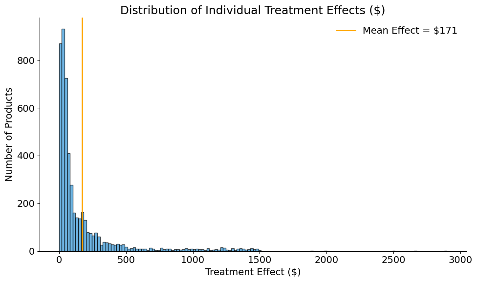
Individual treatment effects

Because we have both potential outcomes, we can compute true individual treatment effects \(\delta_i = Y_i^1 - Y_i^0\):

# Individual treatment effects: delta_i = Y^1_i - Y^0_i
confounded_products["delta"] = confounded_products["Y1"] - confounded_products["Y0"]
print_ite_summary(confounded_products["delta"])

Individual Treatment Effects:
  Mean: $23.40
  Std:  $123.86
  Min:  $0.00
  Max:  $2,317.30

plot_individual_effects_distribution(
    confounded_products["delta"],
    title="Distribution of Individual Treatment Effects ($)",
)

True population parameters

# True ATE, ATT, ATC (we know both potential outcomes for all units)
ATE_true = confounded_products["delta"].mean()
mean_effect = confounded_products.groupby("D")["delta"].mean()
ATT_true = mean_effect[1]
ATC_true = mean_effect[0]

print(f"True ATE: ${ATE_true:,.2f}")
print(f"True ATT: ${ATT_true:,.2f}")
print(f"True ATC: ${ATC_true:,.2f}")

True ATE: $23.40
True ATT: $5.86
True ATC: $30.92

Verifying the bias decomposition

In Part I we derived that the naive estimator decomposes as:

\[\hat{\delta}_{\text{naive}} = \text{ATE} + \underbrace{E[Y^0 \mid D=1] - E[Y^0 \mid D=0]}_{\text{Baseline Bias}} + \underbrace{E[\delta \mid D=1] - E[\delta]}_{\text{Differential Treatment Effect Bias}}\]

Because the simulator gives us \(Y^0\) and \(\delta\) for every product, we can first measure how far the naive estimate is from the truth, and then verify the decomposition numerically:

print_naive_estimator(
    mean_observed[1],
    mean_observed[0],
    ATE_true,
    title="Naive Estimator (Quality-Based Selection)",
)

Naive Estimator (Quality-Based Selection):
  E[Y | D=1] = $17.58
  E[Y | D=0] = $61.85
  Naive estimate = $-44.27

True ATE = $23.40
Bias = $-67.67

# Baseline bias: E[Y^0 | D=1] - E[Y^0 | D=0]
mean_baseline = confounded_products.groupby("D")["Y0"].mean()
baseline_bias = mean_baseline[1] - mean_baseline[0]

# Differential treatment effect bias: E[delta | D=1] - E[delta]
differential_effect_bias = ATT_true - ATE_true

print_bias_decomposition(baseline_bias, differential_effect_bias, naive_estimate, ATE_true)

Bias Decomposition:
  Baseline bias:                $-50.13  (treated have lower Y0)
  Differential treatment effect: $-17.54
  ────────────────────────────────────────
  Total bias:                   $-67.67

Actual bias (Naive - ATE):      $-67.67

Why does the naive estimate fail?

The naive estimate gets even the sign wrong, because both bias terms push it down:

• Baseline bias < 0: the company selected its struggling products for treatment. Treated products would have earned less than control products even without treatment: \(E[Y^0 \mid D=1] < E[Y^0 \mid D=0]\).

• Differential treatment effect bias < 0: the effect is proportional (a 50% revenue boost), so low-revenue products gain fewer dollars. The treated products benefit less than the average product: \(\text{ATT} < \text{ATE}\).

The company’s sensible decision to target its weakest products is exactly what makes the naive comparison misleading.

5. Randomization recovers the truth

In Part I we showed that under randomization, \((Y^1, Y^0) \perp\!\!\!\perp D\), which eliminates selection bias and makes the naive estimator unbiased. We now demonstrate this by using the simulator’s enrichment pipeline to assign treatment randomly to 30% of products. It works on the same 5,000 products with the same 50% boost, now applied to quantity sold, so its results are directly comparable to the quality-based selection above.

Treatment effect configuration

The enrichment pipeline applies a quantity_boost to randomly selected products:

!cat "config_enrichment_random.yaml"

IMPACT:
  FUNCTION: quantity_boost
  PARAMS:
    effect_size: 0.5
    enrichment_fraction: 0.3
    enrichment_start: "2024-11-15"
    seed: 42

Code(inspect.getsource(quantity_boost), language="python")

def quantity_boost(metrics: list, **kwargs) -> tuple:
    """
    Boost ordered units by a percentage for enriched products.

    Args:
        metrics: List of metric record dictionaries
        **kwargs: Parameters including:
            - effect_size: Percentage increase in ordered units (default: 0.5 for 50% boost)
            - enrichment_fraction: Fraction of products to enrich (default: 0.3)
            - enrichment_start: Start date of enrichment (default: "2024-11-15")
            - seed: Random seed for product selection (default: 42)

    Returns:
        Tuple of (treated_metrics, potential_outcomes_df):
            - treated_metrics: List of modified metric dictionaries with treatment applied
            - potential_outcomes_df: DataFrame with Y0_revenue and Y1_revenue for all products
    """
    effect_size = kwargs.get("effect_size", 0.5)
    enrichment_fraction = kwargs.get("enrichment_fraction", 0.3)
    enrichment_start = kwargs.get("enrichment_start", "2024-11-15")
    seed = kwargs.get("seed", 42)

    rng = np.random.default_rng(seed)

    unique_products = sorted(set(record["product_id"] for record in metrics))
    n_enriched = int(len(unique_products) * enrichment_fraction)
    enriched_product_ids = set(rng.choice(unique_products, size=n_enriched, replace=False))

    treated_metrics = []
    potential_outcomes = {}  # {(product_id, date): {'Y0_revenue': x, 'Y1_revenue': y}}
    start_date = datetime.strptime(enrichment_start, "%Y-%m-%d")

    for record in metrics:
        record_copy = copy.deepcopy(record)
        product_id = record_copy["product_id"]
        record_date_str = record_copy["date"]
        record_date = datetime.strptime(record_date_str, "%Y-%m-%d")

        is_enriched = product_id in enriched_product_ids
        record_copy["enriched"] = is_enriched

        # Calculate Y(0) - baseline revenue (no treatment)
        y0_revenue = record_copy["revenue"]

        # Calculate Y(1) - revenue if treated (for ALL products)
        unit_price = record_copy.get("unit_price", record_copy.get("price"))
        if record_date >= start_date:
            original_quantity = record_copy["ordered_units"]
            boosted_quantity = _boost_units(original_quantity, effect_size, rng)
            y1_revenue = round(boosted_quantity * unit_price, 2)
        else:
            # Before treatment start, Y(1) = Y(0)
            y1_revenue = y0_revenue

        # Store potential outcomes for ALL products
        key = (product_id, record_date_str)
        potential_outcomes[key] = {"Y0_revenue": y0_revenue, "Y1_revenue": y1_revenue}

        # Apply factual outcome (only for treated products)
        if is_enriched and record_date >= start_date:
            _apply_boost(record_copy, boosted_quantity, y1_revenue)

        treated_metrics.append(record_copy)

    # Build potential outcomes DataFrame
    potential_outcomes_df = pd.DataFrame(
        [
            {
                "product_identifier": pid,
                "date": d,
                "Y0_revenue": v["Y0_revenue"],
                "Y1_revenue": v["Y1_revenue"],
            }
            for (pid, d), v in potential_outcomes.items()
        ]
    )

    return treated_metrics, potential_outcomes_df

# Apply random treatment using enrichment pipeline
enrich("config_enrichment_random.yaml", job_info)

results = load_job_results(job_info)
metrics_enriched = results["enriched"]
potential_outcomes = results["potential_outcomes"]

print(f"Baseline revenue: ${results['metrics']['revenue'].sum():,.0f}")
print(f"Enriched revenue: ${metrics_enriched['revenue'].sum():,.0f}")

Baseline revenue: $234,038
Enriched revenue: $264,539

# Build full information DataFrame: both potential outcomes plus the observed assignment
full_info_df = potential_outcomes.merge(
    metrics_enriched[["product_identifier", "enriched", "revenue"]],
    on="product_identifier",
).rename(columns={"Y0_revenue": "Y0", "Y1_revenue": "Y1", "enriched": "Treated", "revenue": "Observed"})
full_info_df["delta"] = full_info_df["Y1"] - full_info_df["Y0"]

Covariate balance under randomization

Under random assignment, the distribution of covariates should be similar across treatment and control groups. Before estimating anything, let’s verify this by adding a quality score and checking balance:

Code(inspect.getsource(generate_quality_score), language="python")

def generate_quality_score(revenue, seed=42, noise_std=0.5):
    """
    Generate quality score correlated with revenue.

    Higher revenue products get higher quality scores (realistic assumption:
    good content quality drives higher sales).

    Parameters
    ----------
    revenue : pandas.Series or numpy.ndarray
        Baseline revenue values.
    seed : int or numpy.random.Generator, optional
        Random seed or generator for reproducibility. Default is 42.
    noise_std : float, optional
        Standard deviation of noise. Default is 0.5.

    Returns
    -------
    numpy.ndarray
        Quality scores in range [1, 5].
    """
    rng = np.random.default_rng(seed)

    # Normalize revenue to 0-1 range
    revenue_min = revenue.min()
    revenue_max = revenue.max()
    revenue_normalized = (revenue - revenue_min) / (revenue_max - revenue_min + 1e-6)

    # Map to 1-5 scale with noise
    quality = 1 + 4 * revenue_normalized + rng.normal(0, noise_std, len(revenue))

    return np.clip(quality, 1, 5).round(1)

# Add quality score and check balance under random assignment
full_info_df["quality_score"] = generate_quality_score(full_info_df["Y0"], seed=rng)
full_info_df["D_random"] = full_info_df["Treated"].astype(int)

plot_balance_check(
    full_info_df,
    covariates=["quality_score", "Y0"],
    treatment_col="D_random",
    title="Covariate Balance: Random Assignment (BALANCED)",
)

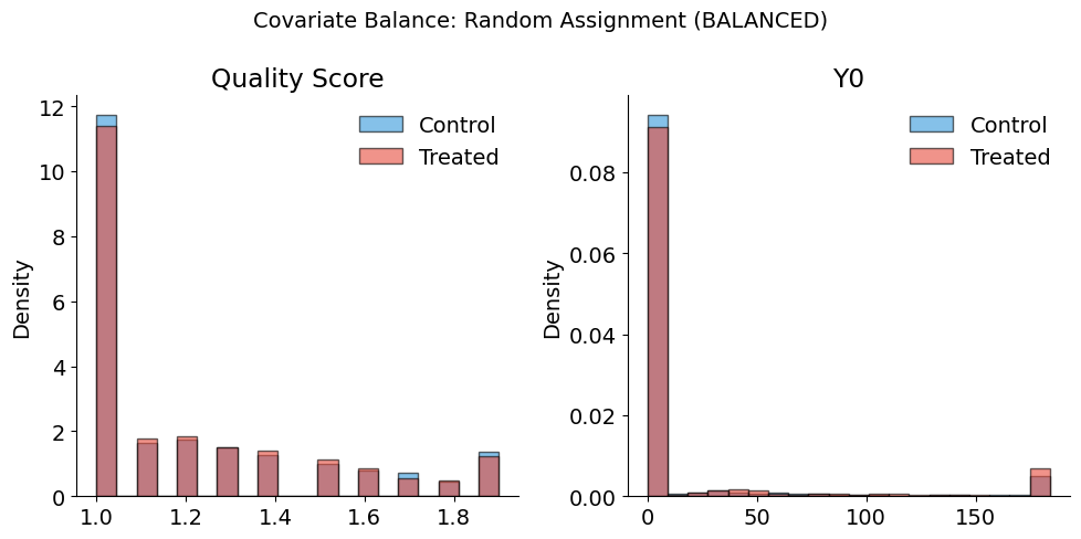
Balance Summary (Mean by Treatment Status):
--------------------------------------------------
quality_score       : Control=    1.23, Treated=    1.23, Diff=   +0.00
Y0                  : Control=   48.09, Treated=   43.82, Diff=   -4.27

Naive estimator under randomization

With balanced groups, the same naive comparison that failed under quality-based selection is now unbiased. Any single estimate still misses the true ATE by some sampling noise, which section 6 examines:

# Naive estimator under random assignment
mean_observed_random = full_info_df.groupby("Treated")["Observed"].mean()
ATE_true_random = full_info_df["delta"].mean()

print_naive_estimator(
    mean_observed_random[True],
    mean_observed_random[False],
    ATE_true_random,
    title="Naive Estimator (Random Assignment)",
)

Naive Estimator (Random Assignment):
  E[Y | D=1] = $64.15
  E[Y | D=0] = $48.09
  Naive estimate = $16.06

True ATE = $23.17
Bias = $-7.11

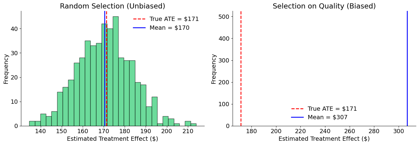
6. Diagnostics & extensions

Monte Carlo: random vs. biased assignment

A single estimate may be close to the truth by luck. To demonstrate the systematic difference between random and biased selection, we run 500 simulations. Random selection draws a new treatment group each time, so it produces a sampling distribution. Selection on quality always treats the same lowest-quality products, so it produces the same biased estimate every time:

# Monte Carlo simulation
# 500 simulations provides stable estimates while keeping runtime reasonable
n_simulations = 500
n_products = len(full_info_df)
n_treat = int(n_products * 0.3)
y1 = full_info_df["Y1"].to_numpy()
y0 = full_info_df["Y0"].to_numpy()

# Random selection: a fresh assignment, and so a fresh estimate, in every simulation
random_estimates = [
    difference_in_means(y1, y0, random_assignment(n_products, n_treat, rng)) for _ in range(n_simulations)
]

# Quality-based selection always treats the same lowest-quality products, so it yields a single estimate
d_quality = full_info_df.index.isin(full_info_df.nsmallest(n_treat, "quality_score").index)
biased_estimate = difference_in_means(y1, y0, d_quality)

print(f"Random selection:  Mean = ${np.mean(random_estimates):,.0f}, Std = ${np.std(random_estimates):,.0f}")
print(f"Quality selection: ${biased_estimate:,.0f}")
print(f"True ATE:          ${ATE_true_random:,.0f}")

Random selection:  Mean = $23, Std = $10
Quality selection: $-42
True ATE:          $23

plot_randomization_comparison(random_estimates, biased_estimate, ATE_true_random)

Uncertainty decreases with sample size

Under random assignment, the naive estimator is unbiased — it is centered on the true ATE. However, any single estimate will differ from the true value due to sampling variability.

The standard error of the difference-in-means estimator decreases at rate \(1/\sqrt{n}\):

\[\text{SE}(\hat{\delta}) \propto \frac{1}{\sqrt{n}}\]

This means quadrupling the sample size cuts uncertainty in half.

# Simulate at different sample sizes, treating half of each sample at random
sample_sizes = [50, 100, 200, 500]
estimates_by_size = {}

for n in sample_sizes:
    estimates = []
    for _ in range(n_simulations):
        sample = full_info_df.iloc[rng.choice(n_products, n, replace=False)]
        d = random_assignment(n, n // 2, rng)
        estimates.append(difference_in_means(sample["Y1"].to_numpy(), sample["Y0"].to_numpy(), d))
    estimates_by_size[n] = estimates

print("Standard Deviation by Sample Size:")
for n in sample_sizes:
    print(f"  n = {n:3d}: ${np.std(estimates_by_size[n]):,.0f}")

Standard Deviation by Sample Size:
  n =  50: $83
  n = 100: $62
  n = 200: $42
  n = 500: $26

plot_sample_size_convergence(sample_sizes, estimates_by_size, ATE_true_random)

7. SUTVA considerations for e-commerce

Our simulation assumes SUTVA holds. In real e-commerce settings, we should consider:

Violation	Example	Implication
Cannibalization	Better content on Product A steals sales from Product B	Interference between products
Market saturation	If ALL products are optimized, relative advantage disappears	Effect depends on treatment prevalence
Budget constraints	Shoppers have fixed budgets; more on A means less on B	Zero-sum dynamics
Search ranking effects	Optimized products rank higher, displacing others	Competitive interference

8. Takeaways for the business

Back to the question: What would be the effect on sales if we improved product content quality?

• Comparing optimized with non-optimized products answers a different question. Because the company optimized its weakest products, the naive comparison says content optimization lowers revenue, while it actually raises it.

• The bias has two sources: treated products would have sold less anyway (baseline bias), and their low baseline revenue means a proportional boost adds fewer dollars (differential treatment effect bias).

• Randomizing which products get optimized removes both, and the simple comparison of means is then unbiased for the true effect. Before a full rollout, the company should test on a random subset large enough for a precise estimate.

Additional resources

• Athey, S. & Imbens, G. W. (2017). The econometrics of randomized experiments. In Handbook of Economic Field Experiments (Vol. 1, pp. 73-140). Elsevier.

• Frölich, M. & Sperlich, S. (2019). Impact Evaluation: Treatment Effects and Causal Analysis. Cambridge University Press.

• Heckman, J. J., Urzua, S. & Vytlacil, E. (2006). Understanding instrumental variables in models with essential heterogeneity. Review of Economics and Statistics, 88(3), 389-432.

• Holland, P. W. (1986). Statistics and causal inference. Journal of the American Statistical Association, 81(396), 945-960.

• Imbens, G. W. (2020). Potential outcome and directed acyclic graph approaches to causality: Relevance for empirical practice in economics. Journal of Economic Literature, 58(4), 1129-1179.

• Imbens, G. W. & Rubin, D. B. (2015). Causal Inference in Statistics, Social, and Biomedical Sciences. Cambridge University Press.

• Rosenbaum, P. R. (2002). Overt bias in observational studies. In Observational Studies (pp. 71-104). Springer.