Download the notebook here! Interactive online version:

Directed Acyclic Graphs

Reference: Causal Inference: The Mixtape, Chapter 3: Directed Acyclic Graphs (pp. 67-117)

This lecture introduces directed acyclic graphs (DAGs) as a tool for reasoning about causal relationships. We apply these concepts using the Online Retail Simulator to answer: Why does our naive analysis suggest content optimization hurts sales?

---

Part I: Theory

This section covers the theoretical foundations of directed acyclic graphs as presented in Cunningham’s Causal Inference: The Mixtape, Chapter 3.

# Standard library
import inspect

# Third-party packages
from IPython.display import Code

# Local imports
from support import draw_police_force_example, simulate_police_force_data

1. Introduction to DAG notation

A directed acyclic graph (DAG) is a visual representation of causal relationships between variables.

Core components

Element	Representation	Meaning
Node	Circle	A random variable
Arrow	Directed edge (→)	Direct causal effect
Path	Sequence of edges	Connection between variables

Key properties

1. Directed: Arrows point in one direction (cause → effect)

2. Acyclic: No variable can cause itself (no loops)

3. Causality flows forward: Time moves in the direction of arrows

What DAGs encode

DAGs encode qualitative causal knowledge:

• What IS happening: drawn arrows

• What is NOT happening: missing arrows (equally important!)

A missing arrow from A to B claims that A does not directly cause B.

Simple DAG: treatment — outcome

2. Paths: direct and backdoor

A path is any sequence of edges connecting two nodes, regardless of arrow direction.

Types of paths

Path Type	Direction	Interpretation
Direct/Causal	D → … → Y	The causal effect we want
Backdoor	D ← … → Y	Spurious correlation (bias!)

The backdoor problem

Backdoor paths create spurious correlations between D and Y:

• They make D and Y appear related even without a causal effect

• This is the graphical representation of selection bias

Path analysis

Path	Type
D → Y	Direct causal path (what we want to estimate)
D ← X → Y	Backdoor path (creates bias)

3. Confounders

A confounder is a variable that:

1. Causes the treatment (D)

2. Causes the outcome (Y)

3. Is NOT on the causal path from D to Y

Observed vs. unobserved

Type	In DAG	Implication
Observed	Solid circle	Can condition on it
Unobserved	Dashed circle	Cannot directly control

Classic example: education and earnings

Consider estimating the return to education:

• Treatment: Years of education

• Outcome: Earnings

• Confounders: Ability, family background, motivation

People with higher ability tend to:

• Get more education (ability → education)

• Earn more regardless of education (ability → earnings)

This creates a backdoor path that inflates naive estimates of education’s effect.

4. Colliders and collider bias

A collider is a variable where two arrows point INTO it:

Key insight about colliders

Colliders have a special property: they naturally BLOCK paths!

Situation	Path Status
Leave collider alone	Path is CLOSED (blocked)
Condition on collider	Path is OPENED (creates bias!)

Why conditioning opens colliders

Conditioning on a collider makes its causes appear correlated, even if they’re independent in the population.

Police use of force: sample selection as a collider

Consider studying whether police use more force against minorities:

• D (Treatment): Minority status

• Y (Outcome): Use of force

• M (Collider): Police stop (sample selection)

• U (Unobserved): Suspicion/perceived threat

The selection problem:

• Minorities are more likely to be stopped (D → M)

• Suspicion affects both stops and force (U → M, U → Y)

• Administrative data only includes stopped individuals

Why this attenuates discrimination estimates:

Among stopped individuals (M = 1), non-minorities (D = 0) who got stopped probably had high suspicion (U)—that’s why they were stopped. Minorities (D = 1) who got stopped could have low or high suspicion, since they face higher stop rates regardless. So within the stopped sample, non-minorities are disproportionately high-suspicion, which correlates with more force (Y). This narrows the apparent gap between groups, masking the true discrimination effect (D → Y).

Simulation setup

Why Show the Simulation Code?

In causal inference, we face a fundamental challenge: we can never directly observe causal effects in real data. When we analyze observational data, we don’t know the true causal structure—we can only make assumptions and hope our methods recover something meaningful. Simulation flips this around. By constructing data with a known causal structure, we create a laboratory where we can verify whether our intuitions and methods actually work. In the code below, we explicitly encoded that minorities face discrimination and that suspicion affects both stops and force. Because we built these relationships ourselves, we know the ground truth. This lets us see—not just theorize—how conditioning on a collider distorts our estimates. Throughout this course, simulation serves as our proving ground: if a method can’t recover known effects in simulated data, we shouldn’t trust it with real data where the stakes are higher and the truth is hidden.

The following function generates synthetic data with the collider structure described above:

Code(inspect.getsource(simulate_police_force_data), language="python")

def simulate_police_force_data(n_population=5000, discrimination_effect=0.3, seed=42):
    """
    Simulate police stop data with collider bias structure.

    The DAG structure:
        Minority (D) → Stop (M) ← Suspicion (U)
        Minority (D) → Force (Y)
        Suspicion (U) → Force (Y)

    Where Stop (M) is the collider that creates sample selection bias.

    Parameters
    ----------
    n_population : int, optional
        Size of the simulated population.
    discrimination_effect : float, optional
        True causal effect of minority status on force (0 = no discrimination).
    seed : int, optional
        Random seed for reproducibility.

    Returns
    -------
    pandas.DataFrame
        DataFrame with columns:
        - minority: minority status (0 or 1)
        - suspicion: suspicion scores
        - is_stopped: boolean stop status
        - force_score: force scores
    """
    rng = np.random.default_rng(seed)

    # Minority status (binary treatment)
    minority = rng.choice([0, 1], size=n_population, p=[0.7, 0.3])

    # Suspicion/perceived threat (unobserved confounder)
    suspicion = rng.normal(50, 15, n_population)

    # Stop probability depends on minority status AND suspicion
    # Minorities are more likely to be stopped (D → M)
    # Higher suspicion leads to more stops (U → M)
    stop_score = (
        0.3 * suspicion  # Suspicion affects stops
        + 15 * minority  # Minorities more likely stopped
        + rng.normal(0, 10, n_population)
    )
    is_stopped = stop_score > np.percentile(stop_score, 70)

    # Force depends on suspicion and minority status
    # True discrimination effect is the parameter
    force_score = (
        0.5 * suspicion  # Higher suspicion → more force (U → Y)
        + discrimination_effect * 20 * minority  # True discrimination (D → Y)
        + rng.normal(0, 10, n_population)
    )

    return pd.DataFrame(
        {
            "minority": minority,
            "suspicion": suspicion,
            "is_stopped": is_stopped,
            "force_score": force_score,
        }
    )

# Simulate population data
police_data = simulate_police_force_data(n_population=5000, discrimination_effect=0.3, seed=42)
police_data

	minority	suspicion	is_stopped	force_score
0	1	33.516132	True	13.429162
1	0	41.880285	True	20.398594
2	1	54.080017	True	29.253445
3	0	40.575200	False	28.486508
4	0	45.824503	False	31.391469
...	...	...	...	...
4995	0	62.382881	False	21.783496
4996	0	23.108498	False	13.325042
4997	0	34.363115	False	30.535183
4998	0	19.034540	False	13.382449
4999	0	36.538923	False	14.671546

5000 rows × 4 columns

# Visualize collider bias
draw_police_force_example(police_data)

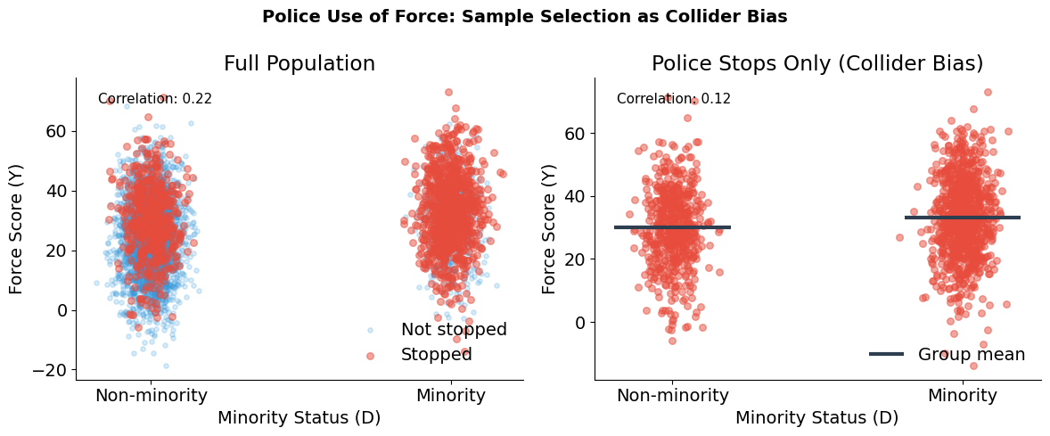
Collider bias in action

True discrimination effect: 30% increase in force for minorities

Sample	Correlation (Minority ↔ Force)
Full population	r = 0.22
Stopped individuals only	r = 0.12

This is collider bias: conditioning on Stop (which depends on both Minority and Suspicion) attenuates the true relationship between minority status and force. The administrative data only includes stopped individuals, so naive analysis of police records underestimates discrimination.

5. The backdoor criterion

The backdoor criterion provides a systematic way to identify what variables to condition on.

Definition

A set of variables \(Z\) satisfies the backdoor criterion relative to \((D, Y)\) if:

1. No variable in \(Z\) is a descendant of \(D\)

2. \(Z\) blocks every backdoor path from \(D\) to \(Y\)

How to block paths

Node Type	To Block	To Open
Non-collider	Condition on it	Leave alone
Collider	Leave alone	Condition on it

Important implications

1. Not all controls are good controls: Conditioning on a collider creates bias

2. Minimal sufficiency: You don’t need to condition on everything—just enough to block backdoors

3. Multiple solutions: Often several valid conditioning sets exist

6. Choosing the right estimand

The backdoor criterion tells us how to block spurious paths. But DAGs also help us reason about a subtler question: which causal effect do we actually want to estimate?

Sometimes a variable is neither a confounder nor a collider—it’s a mediator on the causal path. Whether to condition on it depends on the research question, not on removing bias.

Example: discrimination in hiring

Consider studying gender discrimination in wages:

• Gender → Occupation (women steered to lower-paying jobs)

• Gender → Wages (direct discrimination)

• Occupation → Wages

Question: Should we control for occupation?

Answer: It depends on what effect we want to measure!

• Total effect: Don’t control (captures both direct and indirect discrimination)

• Direct effect: Control for occupation (discrimination within same job)

---

Part II: Application

In Part I we developed the theory of directed acyclic graphs: the backdoor criterion identifies which variables to condition on, d-separation formalizes when conditioning blocks confounding paths, and collider bias shows how conditioning on the wrong variable can create spurious associations.

We now apply DAG concepts to diagnose and solve a confounding problem using simulated data from the Online Retail Simulator. The simulator provides both potential outcomes—an omniscient view that we would not have in real data—enabling numerical verification of the theoretical results from Part I.

From unconditional to conditional comparisons

A naive estimator compares average outcomes between treated and untreated groups:

\[\hat{\delta}_{\text{naive}} = E[Y \mid D=1] - E[Y \mid D=0]\]

This fails when confounders create systematic differences between groups. The treated and untreated have different distributions of background characteristics—we’re comparing apples to oranges.

The backdoor criterion tells us what to condition on. Once we block all backdoor paths, a conditional comparison becomes valid:

\[\hat{\delta}_{\text{conditional}} = E[Y \mid D=1, X] - E[Y \mid D=0, X]\]

The key insight: the problem isn’t the method (comparing means), it’s what we compare. Conditioning on the right variables lets us compare like with like.

# Third-party packages
import pandas as pd
from online_retail_simulator import simulate, load_job_results

# Local imports
from support import (
    compute_effects,
    create_confounded_treatment,
    plot_conditional_comparison,
    plot_confounding_bar,
)

1. Business context: the content optimization paradox

An e-commerce company ran a content optimization program for some of its products. When they analyze the results, they find something puzzling:

Products that received content optimization tend to have LOWER sales than those that didn’t.

The content team is confused. Did their optimization work actually hurt sales?

The underlying reality

What’s actually happening:

• Struggling products (low quality) were selected for content optimization

• Strong products (high quality) sell well without optimization

• Content optimization does increase sales (true causal effect is positive)

But the confounding from product quality creates a negative spurious correlation that overwhelms the positive causal effect. We’ll use DAGs to understand and solve this problem.

Variable	Notation	Description
Treatment	\(D\)	Content optimization (1 = optimized, 0 = not)
Outcome	\(Y\)	Product revenue
Confounder	\(X\)	Product quality (High / Low)
Potential outcomes	\(Y^0, Y^1\)	Revenue without / with optimization

2. Drawing the DAG

Let’s represent this situation graphically:

• Quality (Q): Product quality/strength (unobserved)

• Optimization (D): Content optimization treatment

• Sales (Y): Revenue

Relationships:

1. Quality → Sales (+): Better products sell more

2. Quality → Optimization (−): Struggling products get optimized first

3. Optimization → Sales (+): Optimization increases sales (TRUE causal effect)

Path analysis

Path	Type	Effect
Optimization → Sales	Direct (causal)	True causal effect (+50% revenue boost)
Optimization ← Quality → Sales	Backdoor	Creates negative bias (quality confounding)

3. Generating data with the Online Retail Simulator

We use the Online Retail Simulator to generate realistic e-commerce data. The simulation configuration is defined in "config_simulation.yaml". This gives us products with baseline sales metrics that we can then use to demonstrate confounding.

Data generation process

1. Simulate baseline data: Generate products and their sales metrics

2. Create quality score: Derive a quality measure from baseline revenue (the confounder)

3. Apply confounded treatment: Assign content optimization based on quality (not randomly!)

4. Calculate outcomes: Apply the true treatment effect to get observed sales

# Step 1: Generate baseline data using the simulator
! cat "config_simulation.yaml"

STORAGE:
  PATH: output

RULE:
  PRODUCTS:
    FUNCTION: simulate_products_rule_based
    PARAMS:
      num_products: 5000
      seed: 42

  METRICS:
    FUNCTION: simulate_metrics_rule_based
    PARAMS:
      date_start: "2024-11-15"
      date_end: "2024-11-15"
      sale_prob: 0.7
      seed: 42

PRODUCT_DETAILS:
  FUNCTION: simulate_product_details_mock

# Run simulation
job_info = simulate("config_simulation.yaml")

# Load simulation results
metrics = load_job_results(job_info)["metrics"]

print(f"Metrics records: {len(metrics)}")

Metrics records: 5000

The assignment mechanism

Now we create the confounding structure:

1. Quality: Binary (High/Low) based on median baseline revenue

2. Treatment assignment: Low quality products are more likely to be selected for optimization

This mimics a realistic business scenario where struggling products get prioritized for improvement.

Code(inspect.getsource(create_confounded_treatment), language="python")

def create_confounded_treatment(metrics_df, prob_treat_low=0.6, prob_treat_high=0.2, true_effect=0.5, seed=42):
    """
    Create confounded treatment assignment from raw simulator metrics.

    Aggregates revenue per product, assigns binary quality (High/Low) by median
    split, then assigns treatment confounded by quality: struggling products
    (low quality) are more likely to receive content optimization.

    Parameters
    ----------
    metrics_df : pandas.DataFrame
        Metrics DataFrame with ``product_identifier`` and ``revenue`` columns.
    prob_treat_low : float, optional
        Probability of treatment for low quality products.
    prob_treat_high : float, optional
        Probability of treatment for high quality products.
    true_effect : float, optional
        True causal effect of treatment (proportional increase in revenue).
    seed : int, optional
        Random seed for reproducibility.

    Returns
    -------
    pandas.DataFrame
        DataFrame with columns ``product_identifier``, ``quality``,
        ``baseline_revenue``, ``D``, ``Y0``, ``Y1``, ``Y_observed``.
    """
    quality_df = _create_binary_quality(metrics_df)
    return _apply_confounded_treatment(
        quality_df,
        prob_treat_low=prob_treat_low,
        prob_treat_high=prob_treat_high,
        true_effect=true_effect,
        seed=seed,
    )

# Create confounded treatment assignment
# Low quality products more likely to be optimized
TRUE_EFFECT = 0.5  # 50% revenue boost from optimization

confounded_products = create_confounded_treatment(
    metrics,
    prob_treat_low=0.6,  # 60% of low quality products get optimized
    prob_treat_high=0.2,  # 20% of high quality products get optimized
    true_effect=TRUE_EFFECT,
    seed=42,
)

print(f"Total products: {len(confounded_products)}")
print(f"\nQuality distribution:")
print(confounded_products["quality"].value_counts())
print(f"\nTreatment rates by quality:")
print(confounded_products.groupby("quality")["D"].mean().round(2))
print(f"\n-> Low quality products are MORE likely to be treated (confounding!)")

Total products: 5000

Quality distribution:
quality
Low     2500
High    2500
Name: count, dtype: int64

Treatment rates by quality:
quality
High    0.2
Low     0.6
Name: D, dtype: float64

-> Low quality products are MORE likely to be treated (confounding!)

# Visualize the confounding structure
plot_confounding_bar(confounded_products, TRUE_EFFECT, title="Confounding in Content Optimization")

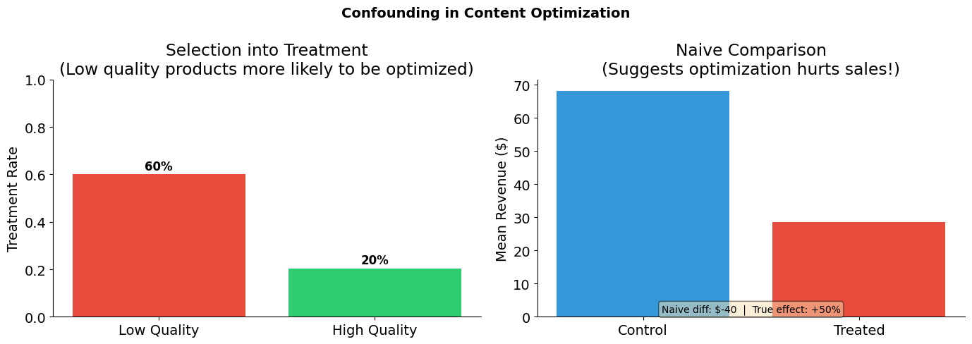
4. What does naive analysis tell us?

Let’s start with what a naive analyst might do: compare average sales between optimized and non-optimized products.

# Naive comparison: unconditional difference in means
treated = confounded_products[confounded_products["D"] == 1]
control = confounded_products[confounded_products["D"] == 0]

naive_estimate = treated["Y_observed"].mean() - control["Y_observed"].mean()

print("Naive Comparison: E[Y|D=1] - E[Y|D=0]")
print("=" * 50)
print(f"Mean revenue (treated):   ${treated['Y_observed'].mean():,.2f}")
print(f"Mean revenue (control):   ${control['Y_observed'].mean():,.2f}")
print(f"Naive estimate:           ${naive_estimate:,.2f}")
print(f"\nTrue effect: +{TRUE_EFFECT:.0%} revenue boost")
print(f"\n-> The naive estimate suggests optimization HURTS sales!")

Naive Comparison: E[Y|D=1] - E[Y|D=0]
==================================================
Mean revenue (treated):   $28.55
Mean revenue (control):   $68.13
Naive estimate:           $-39.59

True effect: +50% revenue boost

-> The naive estimate suggests optimization HURTS sales!

5. How do we apply the backdoor criterion?

Step 1: List all paths from Optimization to Sales

1. Optimization → Sales (direct, causal)

2. Optimization ← Quality → Sales (backdoor, non-causal)

Step 2: Identify which paths are open/closed

• Path 1: Always open (it’s causal)

• Path 2: Open because Quality is a non-collider on this path

Step 3: Find conditioning set to block backdoors

To block the backdoor path Optimization ← Quality → Sales:

• Condition on Quality

This satisfies the backdoor criterion:

• Quality is not a descendant of Optimization

• Conditioning on Quality blocks the backdoor path

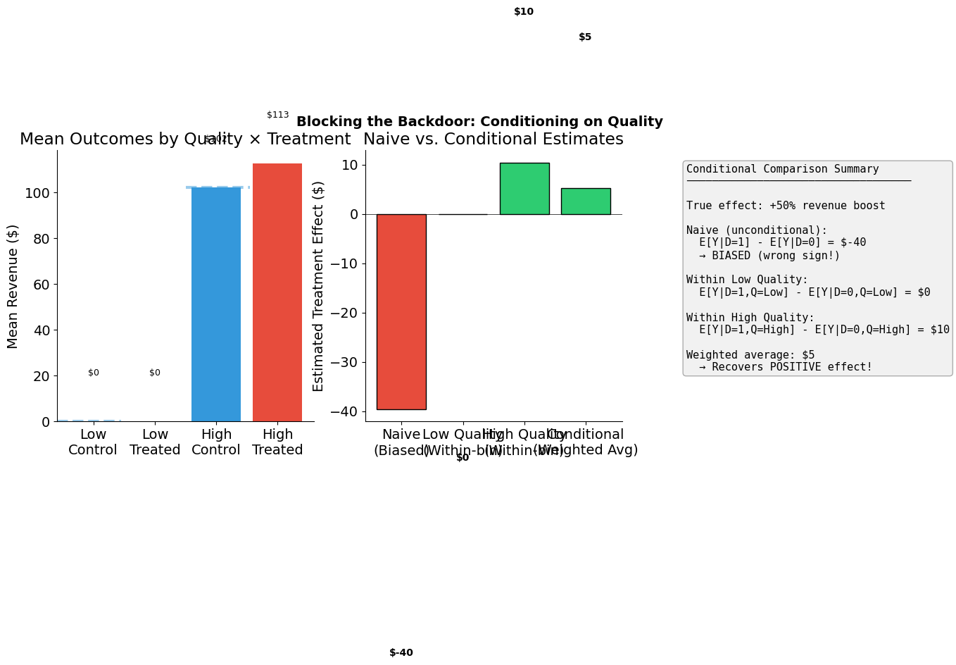
6. How do we recover the causal effect?

We condition on quality by computing treatment effects within each quality bin. This is the conditional comparison in action—we’re comparing products with the same quality level, some optimized and some not.

Low Quality:

\[E[Y \mid D=1, Q=\text{Low}] - E[Y \mid D=0, Q=\text{Low}]\]

High Quality:

\[E[Y \mid D=1, Q=\text{High}] - E[Y \mid D=0, Q=\text{High}]\]

The weighted average of these within-bin effects gives us an unbiased estimate of the treatment effect.

# Compute within-bin treatment effects
effects = compute_effects(confounded_products)

print("Within-Bin Treatment Effects")
print("=" * 50)

for quality in ["Low", "High"]:
    bin_data = confounded_products[confounded_products["quality"] == quality]
    treated_mean = bin_data[bin_data["D"] == 1]["Y_observed"].mean()
    control_mean = bin_data[bin_data["D"] == 0]["Y_observed"].mean()
    n_treated = (bin_data["D"] == 1).sum()
    n_control = (bin_data["D"] == 0).sum()

    print(f"\n{quality} Quality (n={len(bin_data)}):")
    print(f"  E[Y|D=1, Q={quality}] = ${treated_mean:,.2f}  (n={n_treated})")
    print(f"  E[Y|D=0, Q={quality}] = ${control_mean:,.2f}  (n={n_control})")
    print(f"  Effect: ${effects['by_quality'][quality]:,.2f}")

print(f"\n" + "=" * 50)
print(f"Weighted average (conditional estimate): ${effects['conditional']:,.2f}")
print(f"Naive estimate:                          ${effects['naive']:,.2f}")
print(f"True effect: +{TRUE_EFFECT:.0%} revenue boost")
print(f"\n-> Within-bin comparisons recover the POSITIVE effect!")

Within-Bin Treatment Effects
==================================================

Low Quality (n=2500):
  E[Y|D=1, Q=Low] = $0.00  (n=1501)
  E[Y|D=0, Q=Low] = $0.00  (n=999)
  Effect: $0.00

High Quality (n=2500):
  E[Y|D=1, Q=High] = $112.73  (n=509)
  E[Y|D=0, Q=High] = $102.32  (n=1991)
  Effect: $10.41

==================================================
Weighted average (conditional estimate): $5.21
Naive estimate:                          $-39.59
True effect: +50% revenue boost

-> Within-bin comparisons recover the POSITIVE effect!

# Visual summary
plot_conditional_comparison(confounded_products, TRUE_EFFECT)

/home/runner/work/courses-business-decisions/courses-business-decisions/docs/source/measure-impact/02-directed-acyclic-graphs/support.py:458: UserWarning: Tight layout not applied. The bottom and top margins cannot be made large enough to accommodate all Axes decorations.
  plt.tight_layout()

true_effect_dollars = confounded_products["baseline_revenue"].mean() * TRUE_EFFECT

summary = pd.DataFrame(
    {
        "Method": ["Naive (unconditional)", "Conditional (within-bin avg)"],
        "Estimate ($)": [effects["naive"], effects["conditional"]],
        "Error ($)": [
            effects["naive"] - true_effect_dollars,
            effects["conditional"] - true_effect_dollars,
        ],
        "% Error": [
            (effects["naive"] - true_effect_dollars) / true_effect_dollars * 100,
            (effects["conditional"] - true_effect_dollars) / true_effect_dollars * 100,
        ],
    }
)
summary["Estimate ($)"] = summary["Estimate ($)"].map(lambda x: f"${x:,.2f}")
summary["Error ($)"] = summary["Error ($)"].map(lambda x: f"${x:,.2f}")
summary["% Error"] = summary["% Error"].map(lambda x: f"{x:+.1f}%")

print(f"True causal effect: +{TRUE_EFFECT:.0%} revenue boost (${true_effect_dollars:,.2f})")
print()
summary

True causal effect: +50% revenue boost ($24.20)

	Method	Estimate ($)	Error ($)	% Error
0	Naive (unconditional)	$-39.59	$-63.78	-263.6%
1	Conditional (within-bin avg)	$5.21	$-18.99	-78.5%

Additional resources

• Bellemare, M. & Bloem, J. (2020). The paper of how: Estimating treatment effects using the front-door criterion. Working Paper.

• Hünermund, P. & Bareinboim, E. (2019). Causal inference and data-fusion in econometrics. arXiv preprint arXiv:1912.09104.

• Imbens, G. W. (2020). Potential outcome and directed acyclic graph approaches to causality: Relevance for empirical practice in economics. Journal of Economic Literature, 58(4), 1129-1179.

• Manski, C. F. (1995). Identification Problems in the Social Sciences. Harvard University Press.

• Morgan, S. L. & Winship, C. (2014). Counterfactuals and Causal Inference. Cambridge University Press.

• Pearl, J. (2009a). Causality: Models, Reasoning, and Inference (2nd ed.). Cambridge University Press.

• Pearl, J. (2009b). Causal inference in statistics: An overview. Statistics Surveys, 3, 96-146.

• Pearl, J. (2012). The do-calculus revisited. Proceedings of the 28th Conference on Uncertainty in Artificial Intelligence.

• Peters, J., Janzing, D. & Schölkopf, B. (2017). Elements of Causal Inference: Foundations and Learning Algorithms. MIT Press.