Download the notebook here!
Interactive online version: ![]()
Synthetic Control
Reference: Causal Inference: The Mixtape, Chapter 10: Synthetic Control (pp. 469–516)
This lecture introduces the synthetic control method for estimating causal effects in comparative case studies with panel data. We apply these concepts using the Online Retail Simulator to answer: Can synthetic control isolate a campaign’s effect from common time trends that affect all products?
Each application lecture follows the same five-step workflow. We frame a causal question in a business context, simulate data with known ground truth using the Online Retail Simulator, measure the treatment effect — first with a naive approach, then with a causal method — using the Impact Engine, evaluate how well each method recovers the truth, and tune the method’s parameters to understand how configuration choices affect the reliability of causal estimates.

Part I: Theory
1. The comparative case study
Causal inference often involves evaluating the effect of a policy or intervention applied to a single unit—a country, state, firm, or product. When only one unit is treated, traditional methods face a fundamental challenge: there is no randomization and the “sample size” of treated units is exactly one.
The traditional approach is a comparative case study: compare the affected unit to one or more “comparison” units not exposed to the intervention. For example, Card (1990) studied the 1980 Mariel Boatlift—which brought 125,000 Cuban immigrants to Miami—by comparing Miami’s labor market to a set of comparison cities.
The problem with traditional comparative case studies is subjectivity in selecting comparison units. Different researchers might choose different comparison groups and reach different conclusions. Is Atlanta a better comparison for Miami, or is Houston? The answer often depends on the researcher’s judgment, which introduces an element of arbitrariness.
The synthetic control method (Abadie and Gardeazabal 2003; Abadie, Diamond, and Hainmueller 2010) provides a systematic, data-driven approach to this problem. Rather than selecting a single comparison unit, it constructs a synthetic comparison as a weighted average of multiple untreated units.
2. The Synthetic Control estimator
Setup
Suppose we observe \(J + 1\) units over \(T\) time periods. Unit \(j = 1\) receives a treatment or intervention at time \(T_0 + 1\). The remaining \(J\) units (\(j = 2, \ldots, J+1\)) are untreated and form the donor pool.
Let \(Y_{jt}^N\) denote the potential outcome of unit \(j\) at time \(t\) in the absence of treatment, and \(Y_{jt}^I\) the potential outcome under treatment. The causal effect of the intervention on the treated unit at time \(t > T_0\) is:
We observe \(Y_{1t}^I\) directly (the treated unit’s actual outcome after treatment). The challenge is estimating \(Y_{1t}^N\)—what the treated unit’s outcome would have been without the intervention.
Notation bridge. Earlier lectures defined potential outcomes as \(Y^1\) and \(Y^0\) (with vs. without treatment) and the treatment effect as \(\delta_i = Y_i^1 - Y_i^0\). In the synthetic control literature, the convention is \(Y^I\) (intervention) and \(Y^N\) (no intervention), with the treatment effect written \(\alpha_{1t}\). The subscript \(1t\) reflects the panel structure: one treated unit observed across multiple time periods.
The Synthetic Control
The synthetic control method estimates \(Y_{1t}^N\) as a weighted average of the donor units’ outcomes:
where the weights \(W^* = (w_2^*, \ldots, w_{J+1}^*)'\) satisfy:
Non-negativity: \(w_j \geq 0\) for all \(j\)
Sum to one: \(\sum_{j=2}^{J+1} w_j = 1\)
These constraints ensure the synthetic control lies in the convex hull of the donor pool—it is an interpolation, never an extrapolation.
The estimated treatment effect at each post-treatment period is:
Controlling for unobserved factors
Methods like matching and regression rely on selection on observables—they require all confounders to be measured. In comparative case studies, treatment often depends on unobserved factors (political conditions, strategic priorities) that these methods cannot address.
Synthetic control rests on a different identification strategy. Abadie, Diamond, and Hainmueller (2010) model untreated outcomes as:
where \(\lambda_t\) is a common time effect, \(\boldsymbol{\theta}_t\) is a vector of unobserved common factors, and \(\boldsymbol{\mu}_j\) captures unit \(j\)’s factor loadings (its response to those factors). If a weighted combination of donor units reproduces the treated unit’s pre-treatment trajectory, it implicitly matches on the factor loadings \(\boldsymbol{\mu}_j\)—and therefore controls for the unobserved factors \(\boldsymbol{\theta}_t\) in the post-treatment period.
This result depends critically on the length of the pre-treatment period. With few pre-treatment periods, many donor combinations could match the treated trajectory by coincidence. As the pre-treatment period grows, the matching becomes increasingly informative about shared factor structure.
3. Choosing weights
The optimal weights are chosen to make the synthetic control match the treated unit as closely as possible in the pre-treatment period. Let \(k\) denote the number of pre-treatment characteristics used for matching, and define:
\(X_1\) be a \((k \times 1)\) vector of pre-treatment characteristics for the treated unit
\(X_0\) be a \((k \times J)\) matrix of the same characteristics for the donor units
The characteristics in \(X\) typically include pre-treatment outcome values (or averages over pre-treatment subperiods) and other predictors of the outcome.
The optimal weights minimize:
subject to \(w_j \geq 0\) and \(\sum w_j = 1\).
The Role of \(V\)
The matrix \(V\) is a \((k \times k)\) positive semidefinite matrix that reflects the relative importance of different pre-treatment characteristics. It can be:
Approach |
Description |
|---|---|
Researcher-specified |
Set \(V\) based on domain knowledge about which characteristics matter most |
Data-driven |
Choose \(V\) to minimize the mean squared prediction error (MSPE) of the outcome in the pre-treatment period |
Diagonal |
Restrict \(V\) to be diagonal, where each entry reflects one characteristic’s importance |
In practice, the data-driven approach is most common: a nested optimization selects \(V\) in an outer loop to minimize pre-treatment MSPE, and given \(V\), the inner loop solves for the optimal weights \(W^*\).
4. Advantages over regression
A natural alternative to synthetic control is to regress the treated unit’s outcome on the donor units’ outcomes using ordinary least squares. Why prefer synthetic control?
Criterion |
Synthetic Control |
Regression |
|---|---|---|
Interpolation |
Weights are non-negative and sum to 1 \(\rightarrow\) synthetic control lies within the convex hull of donors |
Coefficients are unrestricted \(\rightarrow\) can extrapolate beyond the data |
Transparency |
Weights reveal exactly which units contribute and how much |
Coefficients mix unit contributions with functional form |
Overfitting |
Convexity constraint acts as implicit regularization |
OLS with many predictors can overfit pre-treatment data while predicting post-treatment poorly |
Design focus |
Constructed entirely from pre-treatment data, separating design from analysis |
Same specification used for estimation, inviting specification search |
The interpolation property is particularly important. When the number of potential control units is large relative to the number of pre-treatment periods, OLS will perfectly fit the pre-treatment data (overfitting) but may perform poorly out of sample. The convexity constraint of the synthetic control acts as a natural regularizer, forcing the method to find a meaningful combination of donors rather than an arbitrary one.
5. Inference
Standard inference methods—t-tests, confidence intervals from asymptotic theory—are not appropriate for synthetic control because the treated sample size is one. Instead, Abadie, Diamond, and Hainmueller (2010) propose placebo tests based on permutation inference.
Placebo-in-space tests
The procedure is:
For each unit \(j\) in the donor pool, pretend it was treated and fit a synthetic control using the remaining units as donors
Compute the gap (difference between actual and synthetic) for each placebo unit in the post-treatment period
Compare the treated unit’s gap to the distribution of placebo gaps
If the treated unit’s gap is unusually large relative to the placebo distribution, we have evidence of a genuine treatment effect.
Placebo tests also serve as a check on the unobservables assumption from Section 2. If the treated unit’s post-treatment divergence were driven by an unobserved confounder rather than the treatment, then donor units—exposed to the same unobserved factors but not treated—should show comparable gaps when subjected to placebo analysis. A treated unit whose gap is extreme relative to the placebo distribution provides evidence that the effect is genuine, not an artifact of differential exposure to unobserved shocks.
RMSPE ratios
To formalize the comparison, compute the ratio of post-treatment to pre-treatment root mean squared prediction error for each unit:
where \(\text{RMSPE}_j^{\text{post}}\) measures the post-treatment gap and \(\text{RMSPE}_j^{\text{pre}}\) measures the pre-treatment fit quality.
The ratio adjusts for the fact that some placebo units may have poor pre-treatment fit (large \(\text{RMSPE}^{\text{pre}}\)), which would inflate their post-treatment gaps even without any real effect.
Exact p-Value
The treated unit’s rank among all \(J + 1\) RMSPE ratios gives an exact p-value:
For example, if the treated unit has the highest RMSPE ratio among 20 units (1 treated + 19 donors), the p-value is \(1/20 = 0.05\).
6. Practical considerations
Donor pool selection
The donor pool should contain units that are plausible comparisons—units that could reasonably approximate the treated unit’s trajectory in the absence of treatment. Exclude units that:
Experienced similar interventions or major idiosyncratic shocks during the study period
Are structurally very different from the treated unit (different scale, different market)
Including inappropriate donors adds noise without improving the counterfactual estimate.
Pre-treatment fit quality
The credibility of the synthetic control depends on how well it tracks the treated unit in the pre-treatment period. A large pre-treatment MSPE is a warning sign: if the method cannot reproduce the treated unit’s trajectory before treatment, there is little reason to trust its counterfactual prediction after treatment. A poor fit may indicate that the donor pool does not contain units comparable to the treated unit on unobserved dimensions—undermining the method’s ability to control for selection on unobservables.
As a rule of thumb, the pre-treatment fit should be evaluated both visually (does the synthetic line closely track the treated line?) and quantitatively (is the MSPE small relative to the outcome’s variance?).
When Synthetic Control works best
The method is most effective when:
The pre-treatment period is long enough to reveal the outcome’s dynamics—a requirement for the method’s ability to control for unobserved confounders (Abadie, Diamond, and Hainmueller 2010)
The donor pool contains units whose weighted combination can reproduce the treated unit’s trajectory
The treated unit’s outcome lies within the range of donor outcomes (convex hull condition)
There are no large, idiosyncratic shocks to the treated unit in the pre-treatment period
When these conditions hold, matching on pre-treatment outcomes implicitly controls for heterogeneous responses to unobserved confounders—the key identification result discussed in Section 2.
Part II: Application
In Part I we developed the theory of synthetic control: a weighted average of donor pool units constructs a transparent counterfactual for a single treated unit, with weights constrained to the convex hull of donor outcomes. Inference relies on placebo tests and RMSPE ratios rather than standard errors.
We now apply this method to a product-level panel from our online retail simulation. The simulator provides both potential outcomes—an omniscient view that we would not have in real data—enabling numerical verification of the theoretical results from Part I. A subset of products receives a content optimization campaign starting on a specific date. We observe daily revenue for all products before and after the campaign, then use synthetic control to recover the causal effect for a single showcase product.
Can synthetic control isolate the campaign’s effect from common time trends that affect all products?
[1]:
# Standard library
import inspect

# Third-party packages
from impact_engine_measure import measure_impact, load_results
from IPython.display import Code
from online_retail_simulator import enrich, load_job_results, simulate
import pandas as pd

# Local imports
from support import (
    build_panel,
    compute_ground_truth_att,
    plot_average_fit,
    plot_gap,
    plot_method_comparison,
    plot_placebo_gaps,
    plot_rmspe_ratios,
    plot_treated_vs_synthetic,
    plot_weights,
    run_placebo_tests,
    write_sc_config,
)
1. Business context
An e-commerce company runs a content optimization campaign on 50 products (~10% of its catalog). The campaign improves product listings’ images, descriptions, and search metadata, starting on a specific date. The company observes daily revenue for all 500 products—both the 50 treated and 450 untreated—before and after the campaign launch.
The company wants to know: how much additional daily revenue did the campaign generate?
The challenge is that revenue fluctuates over time for all products due to seasonal patterns, market conditions, and promotional cycles. A simple before-after comparison for a treated product would confound the campaign’s effect with these common time trends. The synthetic control method addresses this by constructing a counterfactual from the untreated products’ trajectories.
Variable |
Notation |
Description |
|---|---|---|
Treated units |
\(j \in \mathcal{T}\) |
50 products receiving content optimization |
Donor pool |
\(j \notin \mathcal{T}\) |
~450 untreated products in the catalog |
Outcome |
\(Y_{jt}\) |
Daily revenue for product \(j\) at time \(t\) |
Treatment time |
\(T_0\) |
Campaign launch date |
Treatment effect |
\(\alpha_{jt}\) |
Additional daily revenue caused by the campaign |
Because we control the data generation process, we observe both each product’s actual revenue and what it would have earned without the campaign. This omniscient view lets us compute the true treatment effect and measure how closely each estimation method recovers it. We demonstrate synthetic control on a single showcase product, then examine aggregate tracking across treated and control groups.
The assignment mechanism
The 50 treated products are selected for the campaign at random—a uniform draw from the full catalog. While random assignment means there is no systematic selection bias by design, any single random draw can produce imbalance between treated and control groups. With only 50 treated products out of 500, chance differences in baseline revenue are common.
At the same time, all 500 products share a common upward time trend in revenue driven by seasonal patterns and market-wide growth. This trend affects treated and untreated products equally but contaminates any before-after comparison for a single product.
A naive before-after estimator for a single treated product captures both the campaign’s true effect and the shared time trend, biasing the estimate upward. The synthetic control method addresses this by constructing a weighted combination of untreated products whose pre-treatment trajectory matches the treated product. Because the donor units experience the same time trends but not the campaign, their weighted average “subtracts out” the common trajectory—isolating the causal effect of content optimization.
[2]:
! cat "config_simulation.yaml"
STORAGE:
  PATH: output

RULE:
  PRODUCTS:
    FUNCTION: simulate_products_rule_based
    PARAMS:
      num_products: 500
      seed: 42

  METRICS:
    FUNCTION: simulate_metrics_rule_based
    PARAMS:
      date_start: "2024-10-01"
      date_end: "2024-12-31"
      sale_prob: 0.7
      seed: 42

PRODUCT_DETAILS:
  FUNCTION: simulate_product_details_mock
[3]:
# Run simulation
job_info = simulate("config_simulation.yaml")
metrics = load_job_results(job_info)["metrics"]

print(f"Metrics records: {len(metrics)}")
print(f"Unique products: {metrics['product_identifier'].nunique()}")
print(f"Date range: {metrics['date'].min()} to {metrics['date'].max()}")
Metrics records: 46000
Unique products: 500
Date range: 2024-10-01 to 2024-12-31
[4]:
! cat "config_enrichment.yaml"
IMPACT:
  FUNCTION: quantity_boost
  PARAMS:
    effect_size: 0.5
    enrichment_fraction: 0.1
    enrichment_start: "2024-11-15"
    seed: 42
[5]:
# Apply enrichment: 50% quantity boost on 10% of products
enriched_job = enrich("config_enrichment.yaml", job_info)
results = load_job_results(enriched_job)
enriched_metrics = results["enriched"]
potential_outcomes = results["potential_outcomes"]

n_treated = enriched_metrics[enriched_metrics["enriched"]]["product_identifier"].nunique()
n_control = enriched_metrics[~enriched_metrics["enriched"]]["product_identifier"].nunique()
print(f"Enriched records: {len(enriched_metrics)}")
print(f"Treated products: {n_treated}")
print(f"Control products: {n_control}")
Enriched records: 46000
Treated products: 50
Control products: 450
[6]:
Code(inspect.getsource(build_panel), language="python")
[6]:
def build_panel(enriched_metrics, potential_outcomes, treatment_date="2024-11-15", trend_slope=5.0):
    """Build analysis-ready panel from enriched simulator output.

    Adds a common upward time trend (so naive before-after estimators are
    visibly biased) and computes counterfactual revenue from the simulator's
    potential outcomes.

    The simulator already produces a balanced panel with one row per product
    per day, so no aggregation or reindexing is needed.

    Parameters
    ----------
    enriched_metrics : pandas.DataFrame
        Enriched metrics from the simulator with product_identifier, date,
        revenue, and enriched columns.
    potential_outcomes : pandas.DataFrame
        Potential outcomes from the simulator with product_identifier, date,
        Y0_revenue, and Y1_revenue columns.
    treatment_date : str, optional
        Date string (YYYY-MM-DD) when the intervention occurs.
    trend_slope : float, optional
        Slope of the common daily time trend added to all products.

    Returns
    -------
    panel : pandas.DataFrame
        Panel with product_identifier, date, revenue, and
        revenue_counterfactual columns.
    treated_products : list of str
        Product identifiers that received treatment.
    control_products : list of str
        Product identifiers in the donor pool.
    """
    panel = enriched_metrics[["product_identifier", "date", "revenue"]].copy()
    panel["date"] = pd.to_datetime(panel["date"])
    panel["product_identifier"] = panel["product_identifier"].astype(str)

    # Merge counterfactual revenue (Y0) from potential outcomes
    po = potential_outcomes[["product_identifier", "date", "Y0_revenue"]].copy()
    po["date"] = pd.to_datetime(po["date"])
    po["product_identifier"] = po["product_identifier"].astype(str)
    panel = panel.merge(po, on=["product_identifier", "date"], how="left")

    # Add common time trend (affects all products equally)
    days_since_start = (panel["date"] - panel["date"].min()).dt.days
    panel["revenue"] = panel["revenue"] + trend_slope * days_since_start
    panel["Y0_revenue"] = panel["Y0_revenue"] + trend_slope * days_since_start

    # Counterfactual: Y0 for all products (what revenue would be without treatment)
    panel["revenue_counterfactual"] = panel["Y0_revenue"]
    panel = panel.drop(columns=["Y0_revenue"])

    # Identify treated vs control products
    products = sorted(panel["product_identifier"].unique())
    treated_products = sorted(
        enriched_metrics[enriched_metrics["enriched"]]["product_identifier"].astype(str).unique().tolist()
    )
    control_products = sorted([p for p in products if p not in treated_products])

    return panel, treated_products, control_products
[7]:
Code(inspect.getsource(compute_ground_truth_att), language="python")
[7]:
def compute_ground_truth_att(panel, treated_products, treatment_date):
    """Compute the true ATT from known potential outcomes.

    Parameters
    ----------
    panel : pandas.DataFrame
        Panel with revenue and revenue_counterfactual columns.
    treated_products : str or list of str
        Product identifier(s) of the treated unit(s).
    treatment_date : str or pandas.Timestamp
        Treatment date.

    Returns
    -------
    float
        True average treatment effect on the treated in the post period.
    """
    if isinstance(treated_products, str):
        treated_products = [treated_products]
    treatment_date = pd.Timestamp(treatment_date)
    post = panel[(panel["product_identifier"].isin(treated_products)) & (panel["date"] >= treatment_date)]
    return (post["revenue"] - post["revenue_counterfactual"]).mean()
[8]:
# Build analysis panel with common time trend
TREATMENT_DATE = "2024-11-15"

panel, treated_products, control_products = build_panel(
    enriched_metrics, potential_outcomes, treatment_date=TREATMENT_DATE
)

# Pick showcase product: first treated product with above-median revenue
avg_rev = panel.groupby("product_identifier")["revenue"].mean()
treated_avg = avg_rev[avg_rev.index.isin(treated_products)]
SHOWCASE_PRODUCT = sorted(treated_avg[treated_avg >= treated_avg.median()].index)[0]

# Save panel for SC: showcase product + control products only (exclude other treated)
sc_panel = panel[panel["product_identifier"].isin([SHOWCASE_PRODUCT] + control_products)]
sc_panel.to_csv("panel_data.csv", index=False)

# Ground truth for showcase product
true_att = compute_ground_truth_att(panel, SHOWCASE_PRODUCT, TREATMENT_DATE)

print(f"Panel shape: {panel.shape}")
print(f"Products: {panel['product_identifier'].nunique()}")
print(f"  Treated: {len(treated_products)}")
print(f"  Control: {len(control_products)}")
print(f"Showcase product: {SHOWCASE_PRODUCT}")
print(f"True ATT (showcase): ${true_att:,.2f}")
Panel shape: (46000, 4)
Products: 500
  Treated: 50
  Control: 450
Showcase product: B2CKZK05CA
True ATT (showcase): $56.69
2. What does the naive comparison tell us?
As a baseline, we compute a simple before-after difference for the showcase product: compare its average daily revenue in the post-treatment period to its average in the pre-treatment period. We use the Impact Engine with an experiment configuration to run this as an OLS regression of revenue on a post-treatment indicator.
This approach ignores the donor pool entirely. Any change in the treated product’s revenue—whether caused by the campaign or by common time trends—is attributed to the treatment.
[9]:
! cat "config_experiment.yaml"
DATA:
  SOURCE:
    type: file
    CONFIG:
      path: treated_data.csv
      date_column: null
  TRANSFORM:
    FUNCTION: passthrough
    PARAMS: {}

MEASUREMENT:
  MODEL: experiment
  PARAMS:
    formula: "revenue ~ post"
[10]:
# Naive before-after comparison for the showcase product
treated_data = panel[panel["product_identifier"] == SHOWCASE_PRODUCT].copy()
treated_data["post"] = (treated_data["date"] >= pd.Timestamp(TREATMENT_DATE)).astype(int)

# Save for the Impact Engine pipeline
treated_data.to_csv("treated_data.csv", index=False)

naive_job = measure_impact("config_experiment.yaml", storage_url="./output/experiment")
naive_result = load_results(naive_job)
naive_estimate = naive_result.impact_results["data"]["impact_estimates"]["params"]["post"]

print("Naive Before-After Comparison")
print("=" * 50)
print(f"Pre-treatment mean:  ${treated_data[treated_data['post'] == 0]['revenue'].mean():,.2f}")
print(f"Post-treatment mean: ${treated_data[treated_data['post'] == 1]['revenue'].mean():,.2f}")
print(f"Naive estimate:      ${naive_estimate:,.2f}")
print(f"\nTrue ATT:            ${true_att:,.2f}")
print(f"Bias:                ${naive_estimate - true_att:,.2f}")
Naive Before-After Comparison
==================================================
Pre-treatment mean:  $137.33
Post-treatment mean: $415.59
Naive estimate:      $278.26

True ATT:            $56.69
Bias:                $221.57
Why does the naive estimate fail?
The before-after comparison confounds the treatment effect with common time trends. All products in the data experience a shared upward trend in revenue over the study period. The naive estimator attributes this trend entirely to the campaign, biasing the estimate upward.
The synthetic control method solves this problem by constructing a counterfactual from the donor pool. Since the untreated products share the same time trends but were not affected by the campaign, their weighted combination provides a valid counterfactual that “subtracts out” the common trajectory.
3. Synthetic Control with the Impact Engine
The Impact Engine implements the synthetic control method from Part I. It uses pysyncon under the hood to find the optimal donor weights that minimize pre-treatment MSPE and estimates the average treatment effect on the treated (ATT) in the post-treatment period.
Interface-to-theory mapping
YAML Config Field |
Part I Concept |
|---|---|
|
Unit identifier \(j\) in the donor pool (\(j = 2, \ldots, J+1\)) |
|
Time index \(t\) in the panel |
|
Outcome \(Y_{jt}\) for unit \(j\) at time \(t\) |
|
Treated unit \(j=1\) receiving the intervention |
|
Intervention time \(T_0\) splitting pre/post periods |
|
Optimization for weight selection: \(\min \|X_1 - X_0 W\|\) |
[11]:
write_sc_config(SHOWCASE_PRODUCT, TREATMENT_DATE)
! cat "config_synthetic_control.yaml"
DATA:
  SOURCE:
    type: file
    CONFIG:
      path: panel_data.csv
      date_column: null
  TRANSFORM:
    FUNCTION: passthrough
    PARAMS: {}
MEASUREMENT:
  MODEL: synthetic_control
  PARAMS:
    unit_column: product_identifier
    time_column: date
    outcome_column: revenue
    treated_unit: B2CKZK05CA
    treatment_time: '2024-11-15'
    optim_method: Nelder-Mead
    optim_initial: equal
[12]:
# Run the synthetic control pipeline
sc_job = measure_impact("config_synthetic_control.yaml", storage_url="./output/synthetic_control")
sc_result = load_results(sc_job)

sc_data = sc_result.impact_results["data"]
sc_att = sc_data["impact_estimates"]["att"]
sc_se = sc_data["impact_estimates"]["se"]
sc_mspe = sc_data["model_summary"]["mspe"]

print("Synthetic Control Results")
print("=" * 50)
print(f"Estimated ATT:  ${sc_att:,.2f}  (SE: ${sc_se:,.2f})")
print(f"True ATT:       ${true_att:,.2f}")
print(f"Bias:           ${sc_att - true_att:,.2f}")
print(f"\nPre-treatment MSPE: {sc_mspe:,.4f}")
print(f"Control units used: {sc_data['model_summary']['n_control_units']}")
Synthetic Control Results
==================================================
Estimated ATT:  $45.63  (SE: $5.13)
True ATT:       $56.69
Bias:           $-11.06

Pre-treatment MSPE: 3,728.7735
Control units used: 450
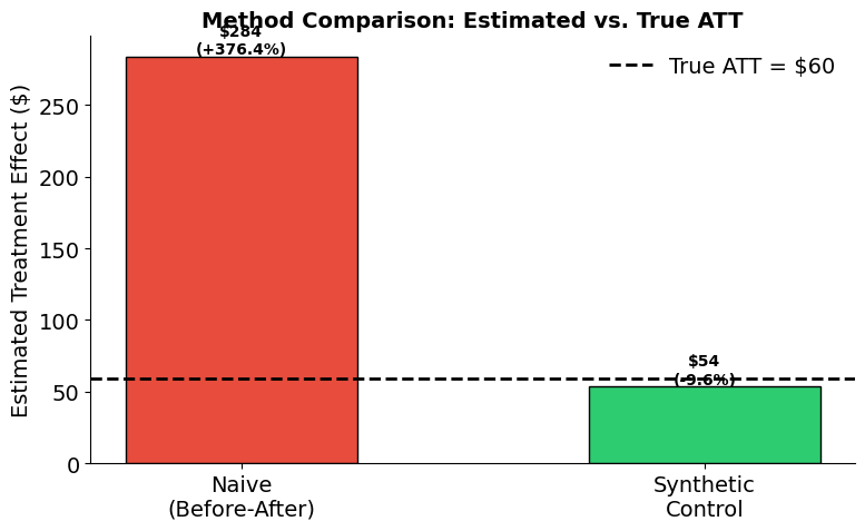
4. Which method best recovers the true effect?
We now compare the naive before-after estimate against the synthetic control estimate. Because we generated the data with known potential outcomes, we can directly measure each method’s bias.
[13]:
plot_method_comparison(
    {"Naive\n(Before-After)": naive_estimate, "Synthetic\nControl": sc_att},
    true_att,
)
[14]:
# Summary statistics table
summary = pd.DataFrame(
    {
        "Method": ["Naive (Before-After)", "Synthetic Control"],
        "Estimate ($)": [naive_estimate, sc_att],
        "Error ($)": [naive_estimate - true_att, sc_att - true_att],
        "% Error": [
            (naive_estimate - true_att) / true_att * 100,
            (sc_att - true_att) / true_att * 100,
        ],
    }
)
summary["Estimate ($)"] = summary["Estimate ($)"].map(lambda x: f"${x:,.2f}")
summary["Error ($)"] = summary["Error ($)"].map(lambda x: f"${x:,.2f}")
summary["% Error"] = summary["% Error"].map(lambda x: f"{x:+.1f}%")

print(f"True ATT: ${true_att:,.2f}")
print()
summary
True ATT: $56.69
[14]:
| Method | Estimate ($) | Error ($) | % Error | |
|---|---|---|---|---|
| 0 | Naive (Before-After) | $278.26 | $221.57 | +390.8% |
| 1 | Synthetic Control | $45.63 | $-11.06 | -19.5% |
5. Diagnostics
Part I Section 6 outlined three practical requirements for credible synthetic control analysis: the donor pool must contain plausible comparisons, the pre-treatment fit must be tight, and the treated unit’s outcome must lie within the convex hull of donor outcomes. We now evaluate each of these using four diagnostics: donor weights, the treated-vs-synthetic time series, the gap plot, and aggregate tracking.
[15]:
plot_weights(sc_data)
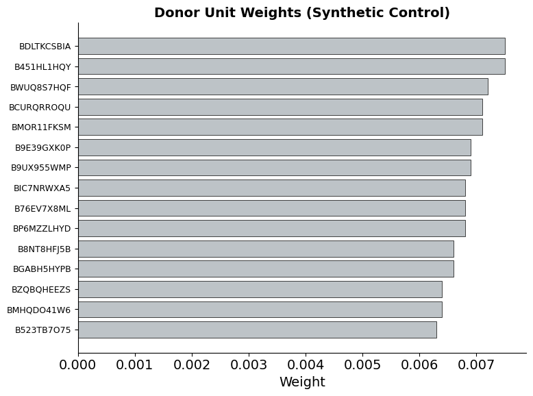
The weights reveal which donor units contribute to the synthetic control and how much. A sparse weight distribution—where only a few donors receive substantial weight—indicates that the method found a small set of products whose revenue trajectories closely resemble the showcase product’s. This is preferable to diffuse weights spread across many donors, which would suggest no single combination fits well.
[16]:
synthetic_ts = plot_treated_vs_synthetic(sc_panel, SHOWCASE_PRODUCT, sc_data, TREATMENT_DATE)
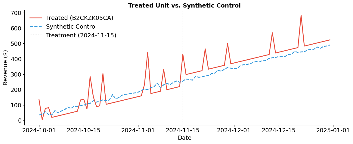
The pre-treatment fit is the most important diagnostic. If the synthetic control closely tracks the treated product before the campaign, then the post-treatment divergence is credible evidence of a treatment effect. A tight pre-treatment fit confirms that the donor pool satisfies the convex hull condition from Part I Section 6—the showcase product’s trajectory can be reproduced as a weighted average of untreated products.
[17]:
plot_gap(sc_panel, SHOWCASE_PRODUCT, synthetic_ts, TREATMENT_DATE)
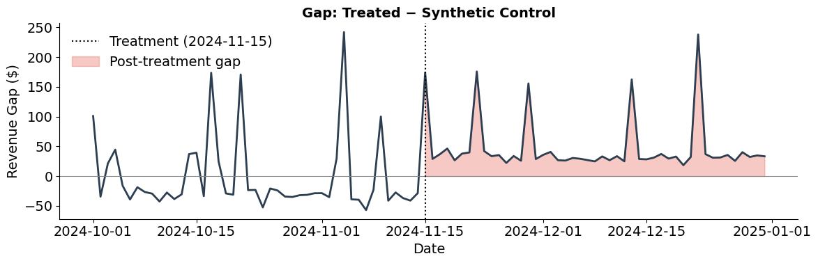
The gap plot isolates the treatment effect over time. Pre-treatment, the gap should fluctuate around zero—confirming a good fit. Post-treatment, a sustained positive gap indicates the campaign increased revenue above what the synthetic control predicts. The shaded area represents the cumulative treatment effect that the synthetic control method recovers.
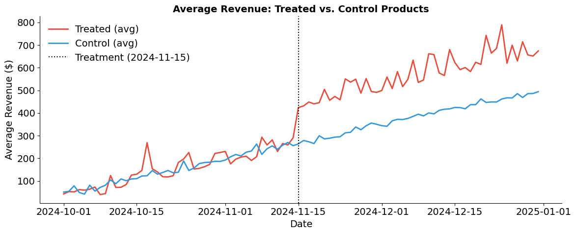
Aggregate tracking
The single-unit plots above show how synthetic control works for one product. But with 50 treated products and 450 controls, we can also examine whether treated and control groups tracked each other at the aggregate level before the campaign.
[18]:
plot_average_fit(panel, treated_products, control_products, TREATMENT_DATE)
6. Placebo inference
Part I Section 5 introduced placebo-in-space tests as the standard approach to inference for synthetic control: fit the method on each donor unit as if it were treated, then compare the treated unit’s gap to the distribution of placebo gaps. If the treated unit’s divergence is extreme relative to what we observe for untreated units, we have evidence of a genuine treatment effect.
We now implement this procedure. For a random subset of donor units, we fit a synthetic control pretending each is the treated unit and compute the RMSPE ratio (post-treatment RMSPE divided by pre-treatment RMSPE) for each. The treated unit’s rank among all RMSPE ratios yields an exact p-value.
[19]:
placebo_results = run_placebo_tests(sc_panel, SHOWCASE_PRODUCT, control_products, TREATMENT_DATE)
  [1/21] B2Q29278DJ — ratio: 1.06
  [2/21] B2V9R52KI1 — ratio: 0.85
  [3/21] B3CQ67HOOU — ratio: 0.80
  [4/21] B4I9L2U2WX — ratio: 1.23
  [5/21] B6E4NMUR4T — ratio: 0.76
  [6/21] BEEJFOLTTA — ratio: 0.95
  [7/21] BEIJR5IXQE — ratio: 0.51
  [8/21] BFKP89F6D0 — ratio: 1.18
  [9/21] BGV7YQPLFV — ratio: 1.02
  [10/21] BH5IVCC1ZN — ratio: 2.02
  [11/21] BL6AP3Z4ON — ratio: 0.99
  [12/21] BNCJYFP1FR — ratio: 1.64
  [13/21] BOMVUUNOAV — ratio: 0.87
  [14/21] BP3DLYEX0X — ratio: 1.29
  [15/21] BQ0172SRIV — ratio: 0.74
  [16/21] BQEBARD8IX — ratio: 2.14
  [17/21] BR8IB0T4DC — ratio: 1.63
  [18/21] BTC8244G7V — ratio: 0.67
  [19/21] BTJZ247EE7 — ratio: 0.73
  [20/21] BY5J1EKKKY — ratio: 1.31
  [21/21] B2CKZK05CA — ratio: 0.94 <- treated
[20]:
plot_placebo_gaps(placebo_results, TREATMENT_DATE)
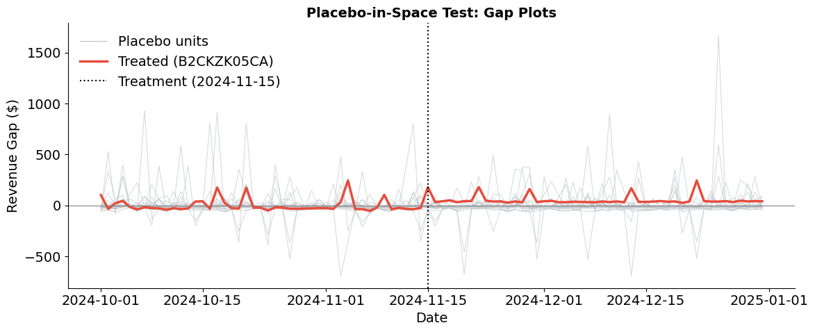
The spaghetti plot overlays the gap (actual minus synthetic) for each placebo unit in gray against the treated unit’s gap in red. Before treatment, all gaps should fluctuate around zero—confirming that the synthetic control fits well for both placebo and treated units. After treatment, the treated unit’s gap should visibly stand out from the placebo distribution. Placebo units, which received no intervention, should show no systematic post-treatment divergence.
[21]:
plot_rmspe_ratios(placebo_results)
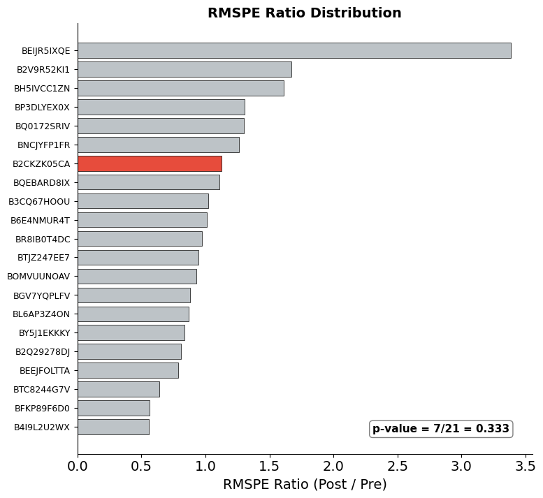
The RMSPE ratio (post-treatment / pre-treatment) formalizes the visual comparison from the spaghetti plot. A large ratio means a unit’s post-treatment divergence is large relative to its pre-treatment fit quality—exactly what we would expect for a genuinely treated unit.
The bar chart ranks all units by their RMSPE ratio, with the treated unit highlighted in red. The exact p-value equals the treated unit’s rank divided by the total number of units: if the treated unit has the highest ratio among \(N\) units, \(p = 1/N\). This implements the permutation-based inference from Part I Section 5, providing a distribution-free test of the null hypothesis that the treatment had no effect.
Additional resources
Abadie, A. & Gardeazabal, J. (2003). The economic costs of conflict: A case study of the Basque Country. American Economic Review, 93(1), 113-132.
Abadie, A., Diamond, A., & Hainmueller, J. (2010). Synthetic control methods for comparative case studies: Estimating the effect of California’s tobacco control program. Journal of the American Statistical Association, 105(490), 493-505.
Abadie, A., Diamond, A., & Hainmueller, J. (2015). Comparative politics and the synthetic control method. American Journal of Political Science, 59(2), 495-510.
Abadie, A. (2021). Using synthetic controls: Feasibility, data requirements, and methodological aspects. Journal of Economic Literature, 59(2), 391-425.
Card, D. (1990). The impact of the Mariel Boatlift on the Miami labor market. Industrial and Labor Relations Review, 43(2), 245-257.
Cunningham, S. (2021). Causal Inference: The Mixtape. Yale University Press. Chapter 10: Synthetic Control.