Download the notebook here!
Interactive online version: ![]()
Matching and Subclassification
Reference: Causal Inference: The Mixtape, Chapter 5: Matching and Subclassification (pp. 175-230)
This lecture introduces methods for causal inference when selection into treatment depends on observed covariates. We apply these concepts using the Online Retail Simulator to answer: Can subclassification and matching recover the true treatment effect when confounding involves multiple continuous covariates?
Each application lecture follows the same five-step workflow. We frame a causal question in a business context, simulate data with known ground truth using the Online Retail Simulator, measure the treatment effect — first with a naive approach, then with a causal method — using the Impact Engine, evaluate how well each method recovers the truth, and tune the method’s parameters to understand how configuration choices affect the reliability of causal estimates.

Part I: Theory
This section covers the theoretical foundations of matching and subclassification as presented in Cunningham’s Causal Inference: The Mixtape, Chapter 5.
1. Selection on observables
In the previous lecture on directed acyclic graphs, we learned that the backdoor criterion tells us which variables to condition on to identify causal effects. When a set of observed covariates \(X\) satisfies the backdoor criterion, we have a situation called selection on observables. This means that treatment assignment, while not random, depends only on variables we can measure and control for.
The conditional independence assumption
The key identifying assumption for all methods in this lecture is the conditional independence assumption (CIA), also known as unconfoundedness or ignorability:
where \(\perp\!\!\!\perp\) denotes statistical independence. This assumption states that, conditional on the observed covariates \(X\), the potential outcomes are independent of treatment assignment. In plain language: once we account for the variables in \(X\), treatment is “as good as random.”
What does this mean in practice? Consider two individuals with identical values of \(X\). Under CIA, the fact that one received treatment and the other did not is essentially random—there are no other factors systematically driving both their treatment status and their outcomes.
Implications of CIA
When CIA holds, the expected potential outcomes are equal across treatment groups for each value of \(X\):
This is powerful because it allows us to use observed outcomes from the control group to estimate the counterfactual for the treatment group (and vice versa) within each stratum defined by \(X\).
Common support
CIA alone is not sufficient for identification. We also need the common support (or overlap) assumption:
This requires that for every value of \(X\), there is a positive probability of being in both the treatment and control groups. Without common support, we cannot compare treated and untreated units with similar characteristics—some regions of the covariate space would have only treated units or only control units.
Assumption |
Formal Statement |
Intuition |
|---|---|---|
CIA |
\((Y^1, Y^0) \perp\!\!\!\perp D \mid X\) |
Treatment is “as good as random” given \(X\) |
Common Support |
\(0 < \Pr(D=1 \mid X) < 1\) |
Both treated and control units exist for all \(X\) |
Together, these assumptions allow us to identify causal effects by comparing outcomes across treatment groups within strata defined by \(X\).
From assumptions to identification
Under CIA and common support, the average treatment effect (ATE) is identified as:
The conditional expectations \(E[Y \mid X, D=1]\) and \(E[Y \mid X, D=0]\) are directly estimable from data. The integral averages these conditional effects over the distribution of \(X\) in the population.
The challenge is how to implement this in practice. With continuous covariates or many discrete covariates, we cannot simply compute separate means for each unique value of \(X\). The methods we discuss below—subclassification and matching—provide practical approaches to this problem.
2. Subclassification
Subclassification is the most direct approach to satisfying the backdoor criterion. The idea is simple: divide the data into strata based on the confounding variable(s), compute treatment effects within each stratum, and then average across strata.
Motivating example: smoking and mortality
Consider a classic problem from epidemiology (simplified from Cochran 1968). We want to estimate the effect of smoking on mortality. The raw data shows that smokers have lower overall death rates than non-smokers—but should we believe this?
The catch is that smokers in this sample are much younger on average. Age is a confounder: it influences both who smokes and mortality risk. Comparing the two groups directly mixes the effect of smoking with the effect of age composition. Subclassification removes this confounding by comparing within age groups.
How subclassification works
The subclassification procedure consists of three steps:
Stratify: Divide the sample into \(K\) mutually exclusive strata based on the covariate(s) \(X\)
Compare: Within each stratum \(k\), compute the difference in mean outcomes between treated and control units
Aggregate: Take a weighted average of the within-stratum effects
For the average treatment effect on the treated (ATT), the estimator is:
where:
\(\bar{Y}^{1k}\) is the mean outcome for treated units in stratum \(k\)
\(\bar{Y}^{0k}\) is the mean outcome for control units in stratum \(k\)
\(N_T^k\) is the number of treated units in stratum \(k\)
\(N_T\) is the total number of treated units
The weights \(\frac{N_T^k}{N_T}\) ensure that the strata contribute to the overall estimate in proportion to how many treated units they contain.
Worked example: age-adjusted mortality rates
The data below (simplified from Cochran 1968) shows death rates per 1,000 person-years for smokers and non-smokers, broken down by age group. The rate columns give the death rate within each age stratum for each group. The count columns show how many people from each group fall into each age stratum—this is where the confounding lives.
Age Group |
Rate (Smokers) |
Rate (Non-Smokers) |
# Smokers |
# Non-Smokers |
|---|---|---|---|---|
20–40 |
20 |
10 |
65 |
10 |
41–70 |
40 |
30 |
25 |
25 |
71+ |
60 |
50 |
10 |
65 |
Total |
100 |
100 |
Notice that smokers are much younger (65% under 40) while non-smokers are much older (65% over 70).
Naive comparison — crude rates weighted by each group’s own age distribution:
The naive difference is \(29 - 41 = -12\), suggesting smokers have lower mortality.
With subclassification — within each age stratum, we compare directly:
Age Group |
Smokers |
Non-Smokers |
Difference |
|---|---|---|---|
20–40 |
20 |
10 |
+10 |
41–70 |
40 |
30 |
+10 |
71+ |
60 |
50 |
+10 |
Within every age group, smokers have a death rate 10 points higher. The naive comparison had the sign wrong because smokers were younger, and younger people die less regardless of smoking status. Subclassification removes this confounding by comparing like with like.
Covariate balance
The goal of subclassification is to achieve covariate balance—making the distribution of confounders similar across treatment and control groups. When the treated and control groups within each stratum have similar covariate values, we say the groups are exchangeable with respect to those covariates.
Balance is the empirical manifestation of the conditional independence assumption. If CIA holds and we have balanced covariates, then any remaining difference in outcomes between treated and control units can be attributed to the treatment effect.
We can check balance by comparing the means (or distributions) of covariates across treatment groups within each stratum. If the means are similar, we have achieved balance on that covariate.
The curse of dimensionality
Subclassification works well when we have one or two discrete covariates. But what happens when we have many covariates, or when covariates are continuous?
This is the curse of dimensionality. As the number of covariates \(K\) grows, the number of strata grows exponentially. With just two binary covariates, we have \(2^2 = 4\) strata. With ten binary covariates, we have \(2^{10} = 1,024\) strata.
The problem is that our sample size doesn’t grow with the number of strata. As strata multiply:
Many strata become empty (no observations)
Many strata have observations of only one type (all treated or all control)
Even strata with both types may have very few observations, leading to imprecise estimates
When a stratum contains only treated units or only control units, we have a common support violation—we cannot estimate the treatment effect in that stratum because we lack a comparison group.
This limitation motivates the methods we discuss next: matching, which provides a more flexible approach to achieving covariate balance.
3. Exact matching
Matching takes a different approach to the identification problem. Instead of stratifying the data and computing within-stratum means, matching directly imputes the missing counterfactual for each treated unit by finding a similar control unit.
The matching idea
Recall the fundamental problem of causal inference: for each treated unit \(i\), we observe \(Y_i^1\) but not \(Y_i^0\). The treatment effect for unit \(i\) is \(\delta_i = Y_i^1 - Y_i^0\), but we can only observe half of this difference.
Matching addresses this by finding a control unit \(j\) with covariate values identical (or very similar) to unit \(i\). Under CIA, this control unit’s outcome \(Y_j\) serves as a valid estimate of unit \(i\)’s counterfactual outcome \(Y_i^0\).
For exact matching, we require that the matched control has exactly the same covariate values:
where \(j(i)\) denotes the control unit matched to treated unit \(i\).
The matching estimator
Once we have found matches, the ATT estimator is simply the average difference between each treated unit’s outcome and its match’s outcome:
This estimator has an intuitive interpretation: for each treated unit, we estimate its individual treatment effect by comparing its outcome to what a similar untreated unit achieved. We then average these individual effects.
Note that this is an estimator of the ATT, not the ATE, because we are averaging over the treated units only. Each treated unit gets equal weight, and the implicit weighting reflects the distribution of \(X\) among the treated.
Example: job training and earnings
Consider a job training program where we want to estimate the effect on earnings. We have data on 5 trainees and 8 non-trainees, with age as the only covariate.
Trainees:
Unit |
Age |
Earnings |
|---|---|---|
1 |
18 |
$9,500 |
2 |
24 |
$11,000 |
3 |
27 |
$11,750 |
4 |
29 |
$12,250 |
5 |
33 |
$13,250 |
Mean |
26.2 |
$11,550 |
Non-Trainees:
Unit |
Age |
Earnings |
|---|---|---|
1 |
40 |
$13,500 |
2 |
24 |
$9,300 |
3 |
44 |
$14,500 |
4 |
18 |
$7,800 |
5 |
29 |
$10,500 |
6 |
33 |
$11,550 |
7 |
27 |
$10,100 |
8 |
47 |
$15,550 |
Mean |
32.8 |
$11,600 |
The naive comparison suggests the program has no effect: trainees earn slightly less on average ($11,550 vs $11,600). But notice that trainees are younger on average (26.2 vs 32.8 years). Since earnings typically rise with age, this comparison is confounded—the non-trainee group includes older, higher-earning individuals who pull up the control mean.
Creating the matched sample
For exact matching on age, we search the non-trainee table for a control unit with the same age as each trainee:
Trainee (Unit) |
Age |
Trainee Earnings |
Match (Unit) |
Match Earnings |
|---|---|---|---|---|
1 |
18 |
$9,500 |
4 |
$7,800 |
2 |
24 |
$11,000 |
2 |
$9,300 |
3 |
27 |
$11,750 |
7 |
$10,100 |
4 |
29 |
$12,250 |
5 |
$10,500 |
5 |
33 |
$13,250 |
6 |
$11,550 |
After matching, the matched control group has the same age distribution as the trainees. The groups are now balanced on age, and therefore exchangeable with respect to this covariate. Non-trainees 1, 3, and 8 (ages 40, 44, 47) are dropped because no trainee shares their age.
The mean earnings of the matched controls is $9,850, compared to $11,550 for trainees. The matching estimate of the ATT is:
Once we compare trainees to non-trainees of the same age, the program increases earnings by $1,700—an effect that was completely hidden by the naive comparison.
Limitations of exact matching
Exact matching inherits the curse of dimensionality from subclassification. With multiple covariates, finding exact matches becomes increasingly difficult:
With continuous covariates (like age measured in days), exact matches may be impossible
With many discrete covariates, the probability of finding an exact match drops rapidly
Some treated units may have no exact match in the control group
When exact matches cannot be found, we must either:
Drop unmatched treated units (reducing sample size and potentially introducing selection bias)
Use approximate matching, which we discuss next
4. Approximate matching
In practice, exact matches are often unavailable. Approximate matching relaxes the requirement of identical covariate values, instead matching on units that are “close” in some sense.
The need for distance metrics
When we cannot find an exact match, we seek the “nearest” control unit. But what does “nearest” mean when comparing multiple covariates?
With a single covariate, distance is straightforward: the distance between ages 25 and 27 is simply 2 years. But with multiple covariates—say, age and income—we need a way to combine distances across dimensions. Is someone who differs by 2 years in age and $1,000 in income “closer” or “farther” than someone who differs by 5 years in age and $200 in income?
This is where distance metrics come in. A distance metric provides a principled way to measure the overall similarity between two units based on their covariate values.
Distance metrics
The most common distance metrics are:
Euclidean Distance
The standard “straight line” distance in covariate space:
The problem with Euclidean distance is that it treats all covariates equally. If age is measured in years (range 18-65) and income in dollars (range $0-$500,000), income will dominate the distance calculation simply because of its larger scale.
Normalized Euclidean Distance
To address the scale problem, we can standardize each covariate by its variance:
where \(\hat{\sigma}_n^2\) is the sample variance of covariate \(n\). Now a one-standard-deviation difference in any covariate contributes equally to the distance.
Mahalanobis Distance
The most sophisticated option accounts for correlations between covariates:
where \(\hat{\Sigma}_X\) is the sample covariance matrix of the covariates. Mahalanobis distance not only standardizes by variance but also accounts for the correlation structure among covariates.
Comparison of distance metrics
Metric |
Formula |
Advantages |
Disadvantages |
|---|---|---|---|
Euclidean |
\(\sqrt{\sum (X_{ni} - X_{nj})^2}\) |
Simple, intuitive |
Scale-dependent |
Normalized Euclidean |
\(\sqrt{\sum \frac{(X_{ni} - X_{nj})^2}{\sigma_n^2}}\) |
Scale-invariant |
Ignores correlations |
Mahalanobis |
\(\sqrt{(X_i-X_j)'\Sigma^{-1}(X_i-X_j)}\) |
Scale-invariant, accounts for correlations |
Requires invertible covariance matrix |
Nearest neighbor matching
Once we have chosen a distance metric, nearest neighbor matching proceeds as follows:
For each treated unit \(i\), compute the distance to all control units
Select the control unit \(j(i)\) with the smallest distance to unit \(i\)
Use \(Y_{j(i)}\) as the imputed counterfactual for unit \(i\)
The ATT estimator remains:
Matching with multiple neighbors: Sometimes we may want to use more than one control unit as a match. If we find \(M\) nearest neighbors for each treated unit, we average their outcomes:
Using multiple matches reduces variance (more data points) but may increase bias (matches are farther away on average).
Matching discrepancies and bias
With approximate matching, the matched control unit typically does not have exactly the same covariate values as the treated unit: \(X_{j(i)} \neq X_i\). This difference is called the matching discrepancy.
Matching discrepancies introduce bias because the control unit’s outcome reflects not just what the treated unit would have experienced under control, but also any systematic differences associated with having different covariate values.
The key insight is that matching discrepancies tend to shrink as the sample size grows—with more potential controls, we can typically find closer matches. In the limit of an infinite control pool, exact matching becomes feasible and the bias disappears.
In finite samples, researchers should:
Examine the quality of matches by comparing covariate distributions before and after matching
Use covariate balance diagnostics to assess whether matching has successfully balanced the groups
Consider whether remaining imbalances could materially affect the estimated treatment effect
The practical takeaway is that approximate matching is a valuable tool, but researchers should be transparent about match quality and the potential for residual bias.
Part II: Application
In Part I we developed the theory of subclassification and matching: the conditional independence assumption identifies causal effects when treatment depends only on observed covariates, subclassification conditions by stratifying on those covariates, and matching imputes counterfactuals from similar control units.
We now apply these methods to simulated data from the Online Retail Simulator. The simulator provides both potential outcomes—an omniscient view that we would not have in real data—enabling numerical verification of the theoretical results from Part I. We know exactly how treatment was assigned. That knowledge — the assignment mechanism — is what makes causal inference possible. Understanding the assignment mechanism tells us what confounding looks like, why naive comparison fails, and which methods can fix it. We use production-grade implementations from the Impact Engine to apply both methods.
[1]:
# Standard library
import inspect

# Third-party packages
from impact_engine_measure import measure_impact, load_results
from IPython.display import Code
from online_retail_simulator import simulate, load_job_results
import pandas as pd

# Local imports
from support import (
    compute_ground_truth_att,
    create_confounded_treatment_multi,
    plot_balance_love_plot,
    plot_covariate_imbalance,
    plot_method_comparison,
    plot_strata_convergence,
    plot_treatment_rates,
    sweep_strata,
)
1. Business context
We return to the content optimization scenario from the previous lecture. An e-commerce company optimizes product listings to boost sales. In the DAGs lecture, confounding came from a single binary variable (product quality High/Low). Here we face a more realistic setting where the company’s selection of which products to optimize depends on three continuous product characteristics — quality_score, price, and impressions.
Variable |
Notation |
Description |
|---|---|---|
Treatment |
\(D\) |
Content optimization (1 = optimized, 0 = not) |
Outcome |
\(Y\) |
Product revenue |
Covariates |
\(X_1, X_2, X_3\) |
|
Potential outcomes |
\(Y^0, Y^1\) |
Revenue without / with optimization |
2. Data generation
We simulate 5,000 products with a single day of sales data. The simulation produces baseline metrics — including quality_score, price, and impressions — that will serve as the covariates driving the assignment mechanism.
[2]:
! cat "config_simulation.yaml"
STORAGE:
  PATH: output

RULE:
  PRODUCTS:
    FUNCTION: simulate_products_rule_based
    PARAMS:
      num_products: 5000
      seed: 42

  METRICS:
    FUNCTION: simulate_metrics_rule_based
    PARAMS:
      date_start: "2024-11-15"
      date_end: "2024-11-15"
      sale_prob: 0.7
      seed: 42

PRODUCT_DETAILS:
  FUNCTION: simulate_product_details_mock
[3]:
# Run simulation and load results
job_info = simulate("config_simulation.yaml")
metrics = load_job_results(job_info)["metrics"]

print(f"Metrics records: {len(metrics)}")
print(f"Unique products: {metrics['product_identifier'].nunique()}")
Metrics records: 5000
Unique products: 5000
3. The assignment mechanism
The optimization team did not randomly select products for content optimization. Instead, they prioritized struggling products — those with low quality scores, low prices, and few impressions. This is a sensible business strategy: invest resources where the need is greatest.
But this strategic selection has a consequence for causal inference. The treatment and control groups differ systematically before any treatment is applied. Products selected for optimization already had lower baseline revenue — not because optimization hurts them, but because the company targeted products that were struggling on multiple dimensions.
Operationalizing selection with a logistic model
To formalize this selection process, we need a function that maps product characteristics to a treatment probability. The probability must lie in \([0, 1]\), which rules out a simple linear model. Instead, we use the logistic (sigmoid) function:
The logistic function has three key properties: (1) its output is always in \([0, 1]\), (2) when \(z = 0\) the probability is exactly \(0.5\), and (3) the sign of each coefficient \(\beta_k\) determines the direction of its effect — negative coefficients mean that lower covariate values increase treatment probability.
Selection coefficients
In our setting, the covariates are standardized (zero mean, unit variance) so that each contributes on a common scale. The linear index is:
All three coefficients are negative, meaning lower covariate values increase treatment probability. The table below maps each coefficient to its business interpretation:
Covariate |
Coefficient |
Direction |
Business Interpretation |
|---|---|---|---|
|
\(-0.5\) |
Lower quality \(\rightarrow\) higher \(\Pr(\text{treat})\) |
Struggling products prioritized |
|
\(-0.8\) |
Lower price \(\rightarrow\) higher \(\Pr(\text{treat})\) |
Budget products prioritized most strongly |
|
\(-0.3\) |
Fewer impressions \(\rightarrow\) higher \(\Pr(\text{treat})\) |
Low-visibility products slightly prioritized |
From assignment mechanism to identifying assumption
Because this selection process uses only the three observable covariates quality_score, price, and impressions, the conditional independence assumption holds when we condition on them:
There are no unobserved factors driving selection. This is what justifies the conditioning-based methods — subclassification and matching — that we apply below. Both methods work by comparing treated and control products with similar values of \(X\), which is exactly the set of variables that the assignment mechanism operates through.
[4]:
Code(inspect.getsource(create_confounded_treatment_multi), language="python")
[4]:
def create_confounded_treatment_multi(
    metrics_df,
    true_effect=0.5,
    seed=42,
    coef_quality=-0.5,
    coef_price=-0.8,
    coef_impressions=-0.3,
):
    """
    Create confounded treatment assignment based on multiple continuous covariates.

    Aggregates per-product revenue from metrics and uses a logistic model
    on quality_score, price, and impressions to determine treatment
    probability. Products with lower covariate values are more likely
    to receive content optimization, creating confounding on all three
    dimensions simultaneously.

    Parameters
    ----------
    metrics_df : pandas.DataFrame
        Metrics DataFrame with product_identifier, revenue, quality_score,
        price, and impressions columns.
    true_effect : float, optional
        True proportional causal effect of treatment on revenue.
    seed : int, optional
        Random seed for reproducibility.
    coef_quality : float, optional
        Logistic model coefficient for quality_score. Negative values mean
        lower quality increases treatment probability.
    coef_price : float, optional
        Logistic model coefficient for price. Negative values mean lower
        price increases treatment probability.
    coef_impressions : float, optional
        Logistic model coefficient for impressions. Negative values mean
        fewer impressions increases treatment probability.

    Returns
    -------
    pandas.DataFrame
        DataFrame with product_identifier, D, Y_observed, Y0, Y1,
        quality_score, price, and impressions columns.
    """
    rng = np.random.default_rng(seed)

    # Aggregate revenue per product (single day, but pattern supports multiple)
    product_revenue = metrics_df.groupby("product_identifier")["revenue"].sum().reset_index()
    product_revenue.columns = ["product_identifier", "baseline_revenue"]

    # Merge continuous covariates from the metrics (one row per product)
    covariates = (
        metrics_df.groupby("product_identifier")[["quality_score", "price", "impressions"]].first().reset_index()
    )
    df = product_revenue.merge(covariates, on="product_identifier")

    # Standardize covariates so each contributes on a common scale
    qs_z = (df["quality_score"] - df["quality_score"].mean()) / df["quality_score"].std()
    price_z = (df["price"] - df["price"].mean()) / df["price"].std()
    imp_z = (df["impressions"] - df["impressions"].mean()) / df["impressions"].std()

    # Logistic model: covariates → treatment probability via sigmoid
    logit = coef_quality * qs_z + coef_price * price_z + coef_impressions * imp_z
    treatment_prob = 1 / (1 + np.exp(-logit))

    df["D"] = (rng.random(len(df)) < treatment_prob).astype(int)

    # Potential outcomes
    df["Y0"] = df["baseline_revenue"]
    df["Y1"] = df["baseline_revenue"] * (1 + true_effect)

    # Observed outcome via switching equation
    df["Y_observed"] = np.where(df["D"] == 1, df["Y1"], df["Y0"])

    return df[["product_identifier", "D", "Y_observed", "Y0", "Y1", "quality_score", "price", "impressions"]]
[5]:
# Apply the assignment mechanism to generate treatment and potential outcomes
TRUE_EFFECT = 0.5  # 50% revenue boost from content optimization

confounded_products = create_confounded_treatment_multi(
    metrics,
    true_effect=TRUE_EFFECT,
    coef_quality=-0.5,
    coef_price=-0.8,
    coef_impressions=-0.3,
    seed=42,
)

# Save for the Impact Engine pipeline
confounded_products.to_csv("confounded_products.csv", index=False)

print(f"Products: {len(confounded_products)}")
print(f"Treated: {confounded_products['D'].sum()} ({confounded_products['D'].mean():.1%})")
print(f"Control: {(1 - confounded_products['D']).sum():.0f} ({1 - confounded_products['D'].mean():.1%})")
Products: 5000
Treated: 2544 (50.9%)
Control: 2456 (49.1%)
[6]:
plot_treatment_rates(confounded_products, ["quality_score", "price", "impressions"])
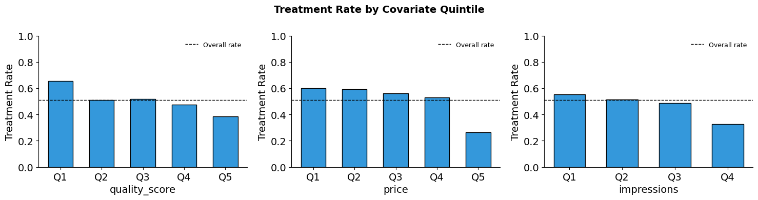
4. What does the naive comparison tell us?
A naive analyst — one who does not know (or ignores) the assignment mechanism — would simply compare mean outcomes across groups, treating the treatment/control split as if it were random.
[7]:
# Naive comparison
treated = confounded_products[confounded_products["D"] == 1]
control = confounded_products[confounded_products["D"] == 0]
naive_estimate = treated["Y_observed"].mean() - control["Y_observed"].mean()

true_att = compute_ground_truth_att(confounded_products)

print("Naive Comparison: E[Y|D=1] - E[Y|D=0]")
print("=" * 50)
print(f"Mean revenue (treated):   ${treated['Y_observed'].mean():,.2f}")
print(f"Mean revenue (control):   ${control['Y_observed'].mean():,.2f}")
print(f"Naive estimate:           ${naive_estimate:,.2f}")
print(f"\nTrue ATT:                 ${true_att:,.2f}")
print(f"Bias:                     ${naive_estimate - true_att:,.2f}")
Naive Comparison: E[Y|D=1] - E[Y|D=0]
==================================================
Mean revenue (treated):   $25.50
Mean revenue (control):   $75.32
Naive estimate:           $-49.82

True ATT:                 $8.50
Bias:                     $-58.32
Why does the naive estimate fail?
The naive estimate is biased because the assignment mechanism selected treated products based on their covariate values. The company chose products with lower quality scores, lower prices, and fewer impressions — and since all three covariates positively predict baseline revenue, the treated group has systematically lower revenue even in the absence of any treatment effect.
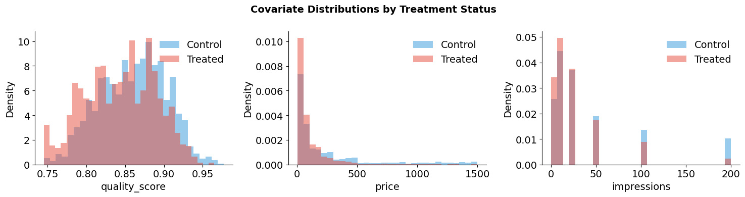
This is negative selection bias: the treated group’s lower baseline pulls down their mean outcome, masking (or reversing) the positive treatment effect. In the language of Part I, the CIA tells us that conditioning on \(X\) would remove this bias. The histograms below show why conditioning is needed — the covariate distributions are shifted between groups, exactly as the assignment mechanism’s negative coefficients predict.
[8]:
plot_covariate_imbalance(confounded_products, ["quality_score", "price", "impressions"])
5. Subclassification with the Impact Engine
The assignment mechanism operates through three continuous covariates. The CIA tells us: condition on these covariates and confounding disappears. Subclassification achieves this by discretizing each covariate into quantile-based bins, creating strata where products within the same bin have similar characteristics. Within each stratum, the assignment mechanism’s influence is approximately removed — products are roughly comparable regardless of treatment status.
With three continuous covariates, the curse of dimensionality from Part I applies directly: with n_strata set to 4, each covariate is split into 4 quantile-based bins, creating \(4^3 = 64\) potential strata — many of which may lack common support. The SubclassificationAdapter from the Impact Engine handles this by dropping strata without both treated and control units.
Configuration-to-theory mapping
The MEASUREMENT.PARAMS fields in the YAML configuration map directly to the components of our causal model. The covariate_columns are the three variables that drive the assignment mechanism — conditioning on them is what makes CIA hold.
YAML Config Field |
Part I Concept |
|---|---|
|
Binary treatment indicator \(D\) |
|
Conditioning set \(X\) from CIA: \((Y^1, Y^0) \perp\!\!\!\perp D \mid X\) |
|
Observed outcome \(Y\) |
|
Number of strata \(K\) in the subclassification estimator |
|
ATT weighting: \(\frac{N_T^k}{N_T}\) per stratum |
[9]:
! cat "config_subclassification.yaml"
DATA:
  SOURCE:
    type: file
    CONFIG:
      path: confounded_products.csv
  TRANSFORM:
    FUNCTION: passthrough
    PARAMS: {}

MEASUREMENT:
  MODEL: subclassification
  PARAMS:
    treatment_column: D
    covariate_columns:
      - quality_score
      - price
      - impressions
    dependent_variable: Y_observed
    n_strata: 4
    estimand: att
[10]:
# Run the subclassification pipeline
sub_job = measure_impact("config_subclassification.yaml", storage_url="./output/subclassification")
sub_result = load_results(sub_job)

sub_estimate = sub_result.impact_results["data"]["impact_estimates"]["treatment_effect"]
n_strata = sub_result.impact_results["data"]["impact_estimates"]["n_strata"]
n_dropped = sub_result.impact_results["data"]["impact_estimates"]["n_strata_dropped"]

print("Subclassification Results")
print("=" * 50)
print(f"Estimated ATT:   ${sub_estimate:,.2f}")
print(f"True ATT:        ${true_att:,.2f}")
print(f"Bias:            ${sub_estimate - true_att:,.2f}")
print(f"\nStrata used: {n_strata}  |  Strata dropped (no common support): {n_dropped}")
Covariate 'impressions': requested 4 bins but got 3 due to duplicate quantile edges.
Subclassification Results
==================================================
Estimated ATT:   $-1.69
True ATT:        $8.50
Bias:            $-10.19

Strata used: 48  |  Strata dropped (no common support): 0
[11]:
# Examine stratum-level details
sub_result.model_artifacts["stratum_details"]
[11]:
| stratum | n_treated | n_control | mean_treated | mean_control | effect | |
|---|---|---|---|---|---|---|
| 0 | 0_0_0 | 129 | 33 | 0.000000 | 0.000000 | 0.000000 |
| 1 | 0_0_1 | 51 | 17 | 0.000000 | 0.000000 | 0.000000 |
| 2 | 0_0_2 | 39 | 18 | 34.706154 | 32.949444 | 1.756709 |
| 3 | 0_1_0 | 158 | 50 | 0.000000 | 0.000000 | 0.000000 |
| 4 | 0_1_1 | 54 | 21 | 0.000000 | 0.000000 | 0.000000 |
| 5 | 0_1_2 | 67 | 21 | 71.570373 | 56.489048 | 15.081326 |
| 6 | 0_2_0 | 114 | 51 | 0.000000 | 0.000000 | 0.000000 |
| 7 | 0_2_1 | 52 | 18 | 0.000000 | 0.000000 | 0.000000 |
| 8 | 0_2_2 | 41 | 28 | 149.761463 | 129.900714 | 19.860749 |
| 9 | 0_3_0 | 53 | 104 | 0.000000 | 0.000000 | 0.000000 |
| 10 | 0_3_1 | 19 | 61 | 0.000000 | 0.000000 | 0.000000 |
| 11 | 0_3_2 | 10 | 57 | 719.091000 | 1081.924386 | -362.833386 |
| 12 | 1_0_0 | 90 | 39 | 0.000000 | 0.000000 | 0.000000 |
| 13 | 1_0_1 | 49 | 19 | 0.000000 | 0.000000 | 0.000000 |
| 14 | 1_0_2 | 39 | 24 | 29.828846 | 25.273750 | 4.555096 |
| 15 | 1_1_0 | 93 | 52 | 0.000000 | 0.000000 | 0.000000 |
| 16 | 1_1_1 | 44 | 25 | 0.000000 | 0.000000 | 0.000000 |
| 17 | 1_1_2 | 34 | 20 | 64.773971 | 50.433000 | 14.340971 |
| 18 | 1_2_0 | 106 | 65 | 0.000000 | 0.000000 | 0.000000 |
| 19 | 1_2_1 | 53 | 36 | 0.000000 | 0.000000 | 0.000000 |
| 20 | 1_2_2 | 44 | 43 | 174.594545 | 113.683023 | 60.911522 |
| 21 | 1_3_0 | 61 | 133 | 0.000000 | 0.000000 | 0.000000 |
| 22 | 1_3_1 | 28 | 80 | 0.000000 | 0.000000 | 0.000000 |
| 23 | 1_3_2 | 22 | 63 | 381.521591 | 638.237619 | -256.716028 |
| 24 | 2_0_0 | 111 | 73 | 0.000000 | 0.000000 | 0.000000 |
| 25 | 2_0_1 | 38 | 36 | 0.000000 | 0.000000 | 0.000000 |
| 26 | 2_0_2 | 40 | 46 | 22.830000 | 20.156087 | 2.673913 |
| 27 | 2_1_0 | 85 | 80 | 0.000000 | 0.000000 | 0.000000 |
| 28 | 2_1_1 | 58 | 41 | 0.000000 | 0.000000 | 0.000000 |
| 29 | 2_1_2 | 27 | 46 | 63.715000 | 59.656739 | 4.058261 |
| 30 | 2_2_0 | 84 | 61 | 0.000000 | 0.000000 | 0.000000 |
| 31 | 2_2_1 | 38 | 26 | 0.000000 | 0.000000 | 0.000000 |
| 32 | 2_2_2 | 32 | 32 | 154.247344 | 99.218750 | 55.028594 |
| 33 | 2_3_0 | 59 | 89 | 0.000000 | 0.000000 | 0.000000 |
| 34 | 2_3_1 | 18 | 42 | 0.000000 | 0.000000 | 0.000000 |
| 35 | 2_3_2 | 15 | 52 | 434.744000 | 555.838269 | -121.094269 |
| 36 | 3_0_0 | 88 | 84 | 0.000000 | 0.000000 | 0.000000 |
| 37 | 3_0_1 | 43 | 54 | 0.000000 | 0.000000 | 0.000000 |
| 38 | 3_0_2 | 32 | 59 | 21.620156 | 21.124915 | 0.495241 |
| 39 | 3_1_0 | 71 | 70 | 0.000000 | 0.000000 | 0.000000 |
| 40 | 3_1_1 | 31 | 37 | 0.000000 | 0.000000 | 0.000000 |
| 41 | 3_1_2 | 23 | 41 | 81.556957 | 57.834878 | 23.722078 |
| 42 | 3_2_0 | 74 | 103 | 0.000000 | 0.000000 | 0.000000 |
| 43 | 3_2_1 | 26 | 53 | 0.000000 | 0.000000 | 0.000000 |
| 44 | 3_2_2 | 21 | 49 | 126.841429 | 129.476735 | -2.635306 |
| 45 | 3_3_0 | 39 | 83 | 0.000000 | 0.000000 | 0.000000 |
| 46 | 3_3_1 | 19 | 47 | 0.000000 | 0.000000 | 0.000000 |
| 47 | 3_3_2 | 22 | 74 | 301.727045 | 344.314730 | -42.587684 |
How many strata? Bias vs. the curse of dimensionality
The choice of n_strata controls the bias-variance tradeoff discussed in Part I. With few strata per covariate, each bin is wide — treated and control products within the same stratum may still differ substantially, leaving residual confounding. Increasing the number of strata narrows the bins and reduces this within-stratum bias.
But with three covariates, the total number of strata grows as \(K^3\). As \(K\) increases, many strata end up with only treated or only control products — a common support violation. These strata must be dropped, meaning the estimate is based on an increasingly selective subset of the data. The figure below sweeps across different values of \(K\) to visualize both effects simultaneously.
[12]:
# Sweep across strata counts to show convergence and common support loss
covariates = ["quality_score", "price", "impressions"]
convergence_df = sweep_strata(confounded_products, [2, 3, 4, 5, 7, 10, 15, 20], covariates)
plot_strata_convergence(convergence_df, true_att)
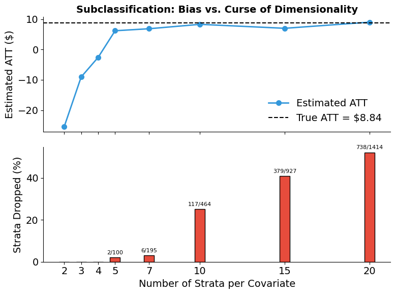
The top panel shows the estimated ATT converging toward the true effect as \(K\) increases — finer bins reduce within-stratum confounding, just as the theory predicts. But the bottom panel reveals the cost: the fraction of strata dropped for lack of common support rises sharply. With three covariates, the total strata grow as \(K^3\), and the fixed sample of 5,000 products cannot populate them all. This is the curse of dimensionality in action — more strata improve bias but eventually exhaust the data.
6. Nearest neighbor matching with the Impact Engine
Subclassification discretizes the covariate space into bins, which can be lossy — two products in the same bin may still differ substantially on the covariates that drove treatment selection. Matching takes a different approach to the same problem.
Instead of binning, matching directly implements the CIA logic: for each treated product, find a control product with the most similar covariate profile. If the match is close enough, the assignment mechanism’s influence is effectively neutralized — we are comparing two products that would have had nearly the same treatment probability. The NearestNeighbourMatchingAdapter wraps causalml’s NearestNeighborMatch, using a distance metric on the
covariates to find closest matches. Because the three covariates have different scales and different coefficients in the assignment mechanism, the distance metric must account for scale differences.
Configuration-to-theory mapping
The covariate_columns define the dimensions of the distance metric — these must include all variables that drive the assignment mechanism, so that conditional on a close match, treatment is effectively random.
YAML Config Field |
Part I Concept |
|---|---|
|
Binary treatment indicator \(D\) |
|
Dimensions of the distance metric: \(\|X_i - X_j\|\) |
|
Observed outcome \(Y\) |
|
Maximum matching discrepancy threshold (Section 4) |
|
Matching with replacement — bias-variance tradeoff |
|
\(M\) nearest neighbors: \(\frac{1}{M}\sum_{m=1}^{M} Y_{j_m(i)}\) |
[13]:
! cat "config_matching.yaml"
DATA:
  SOURCE:
    type: file
    CONFIG:
      path: confounded_products.csv
  TRANSFORM:
    FUNCTION: passthrough
    PARAMS: {}

MEASUREMENT:
  MODEL: nearest_neighbour_matching
  PARAMS:
    treatment_column: D
    covariate_columns:
      - quality_score
      - price
      - impressions
    dependent_variable: Y_observed
    caliper: 0.2
    replace: true
    ratio: 1
    random_state: 42
[14]:
# Run the nearest-neighbour matching pipeline
nn_job = measure_impact("config_matching.yaml", storage_url="./output/matching")
nn_result = load_results(nn_job)

nn_att = nn_result.impact_results["data"]["impact_estimates"]["att"]
nn_atc = nn_result.impact_results["data"]["impact_estimates"]["atc"]
nn_ate = nn_result.impact_results["data"]["impact_estimates"]["ate"]
nn_att_se = nn_result.impact_results["data"]["impact_estimates"]["att_se"]

print("Nearest Neighbor Matching Results")
print("=" * 50)
print(f"ATT:   ${nn_att:,.2f}  (SE: ${nn_att_se:,.2f})")
print(f"ATC:   ${nn_atc:,.2f}")
print(f"ATE:   ${nn_ate:,.2f}")
print(f"\nTrue ATT: ${true_att:,.2f}")
print(f"Bias:     ${nn_att - true_att:,.2f}")
Nearest Neighbor Matching Results
==================================================
ATT:   $7.04  (SE: $2.77)
ATC:   $13.14
ATE:   $10.04

True ATT: $8.50
Bias:     $-1.46
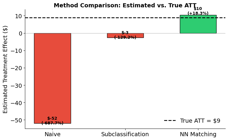
7. Which method best recovers the true effect?
Because we built the assignment mechanism ourselves, we know the true ATT. This lets us verify that conditioning on the covariates that drive treatment selection — via either subclassification or matching — recovers the true causal effect. The naive estimate’s failure confirms that the assignment mechanism creates real confounding; the methods’ success confirms that conditioning on the right variables removes it.
[15]:
plot_method_comparison(
    {"Naive": naive_estimate, "Subclassification": sub_estimate, "NN Matching": nn_att},
    true_att,
)
[16]:
# Summary statistics table
summary = pd.DataFrame(
    {
        "Method": ["Naive", "Subclassification", "NN Matching"],
        "Estimate ($)": [naive_estimate, sub_estimate, nn_att],
        "Error ($)": [naive_estimate - true_att, sub_estimate - true_att, nn_att - true_att],
        "% Error": [
            (naive_estimate - true_att) / true_att * 100,
            (sub_estimate - true_att) / true_att * 100,
            (nn_att - true_att) / true_att * 100,
        ],
    }
)
summary["Estimate ($)"] = summary["Estimate ($)"].map(lambda x: f"${x:,.2f}")
summary["Error ($)"] = summary["Error ($)"].map(lambda x: f"${x:,.2f}")
summary["% Error"] = summary["% Error"].map(lambda x: f"{x:+.1f}%")

print(f"True ATT: ${true_att:,.2f}")
print()
summary
True ATT: $8.50
[16]:
| Method | Estimate ($) | Error ($) | % Error | |
|---|---|---|---|---|
| 0 | Naive | $-49.82 | $-58.32 | -686.0% |
| 1 | Subclassification | $-1.69 | $-10.19 | -119.9% |
| 2 | NN Matching | $7.04 | $-1.46 | -17.2% |
8. Diagnostics & extensions
A key advantage of matching is that we can directly assess whether the method has achieved its goal — removing the assignment mechanism’s influence on covariate distributions. The diagnostics below evaluate covariate balance before and after nearest neighbor matching.
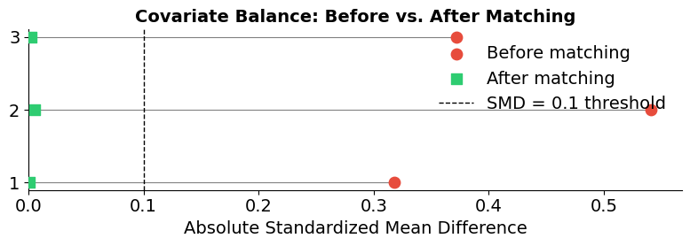
Covariate balance diagnostics
If matching successfully removes the assignment mechanism’s influence, the covariate distributions of matched treated and control groups should be indistinguishable. The standardized mean difference (SMD) measures residual imbalance: the difference in covariate means between groups, normalized by the pooled standard deviation. An SMD below 0.1 suggests that the assignment mechanism’s effect on that covariate has been effectively neutralized.
[17]:
# Print balance tables
balance_before = nn_result.model_artifacts["balance_before"]
balance_after = nn_result.model_artifacts["balance_after"]

print("Balance BEFORE matching:")
print(balance_before)
print("\nBalance AFTER matching:")
print(balance_after)
Balance BEFORE matching:
           Control        Treatment      SMD
0             2456             2544
1    36.11 (49.13)    26.11 (37.58)  -0.2287
2  263.82 (362.16)  111.00 (167.83)  -0.5415
3      0.86 (0.04)      0.84 (0.05)  -0.3713

Balance AFTER matching:
           Control        Treatment      SMD
0             2522             2522
1    25.66 (37.23)    25.66 (37.23)      0.0
2  109.51 (165.51)  110.17 (165.40)    0.004
3      0.84 (0.04)      0.84 (0.04)  -0.0012
[18]:
plot_balance_love_plot(balance_before, balance_after)
Additional resources
Abadie, A. & Imbens, G. (2006). Large sample properties of matching estimators for average treatment effects. Econometrica, 74(1), 235-267.
Abadie, A. & Imbens, G. (2011). Bias-corrected matching estimators for average treatment effects. Journal of Business & Economic Statistics, 29(1), 1-11.
Cochran, W. G. (1968). The effectiveness of adjustment by subclassification in removing bias in observational studies. Biometrics, 24(2), 295-313.
Imbens, G. W. (2004). Nonparametric estimation of average treatment effects under exogeneity: A review. Review of Economics and Statistics, 86(1), 4-29.
Rosenbaum, P. R. (2002). Observational Studies (2nd ed.). Springer.
Rosenbaum, P. R. & Rubin, D. B. (1983). The central role of the propensity score in observational studies for causal effects. Biometrika, 70(1), 41-55.
Stuart, E. A. (2010). Matching methods for causal inference: A review and a look forward. Statistical Science, 25(1), 1-21.